Fairness is becoming a hot topic amongst machine learning researchers and practitioners. The field is aware that their models have a large impact on society and that their predictions are not always beneficial. In a previous blog, Stijn showed how adversarial networks can be used to make fairer predictions. This blog post focuses on the implementation part of things, so that you as a practitioner are able to build your own fair classifiers.
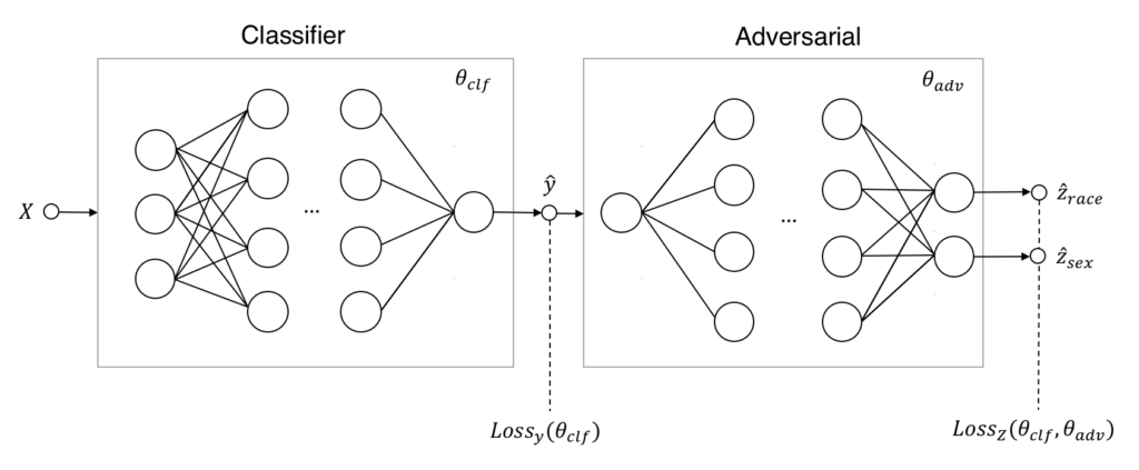
Lets start with a short recap of how adversarial networks can help to battle unfairness. Instead of having only a single classifier that makes predictions \hat{y} with data X, we introduce an adversary that tries to predict if the classifier is unfair for the sensitive attributes Z. The classifier has to compete with the adversary in a zero-sum game: the classifier has to make good predictions but is being penalized if the adversary detects unfair decisions. The end-result of this game is, hopefully, a fair classifier that is also good at predicting.

In the next section, we start by loading the datasets with some PyTorch utilities. After that, we will separately define and pretrain the classifier and adversary. These components are then combined and trained together to give a fair classifier.
Data
Our goal is to predict income levels based on personal attributes, such as age, education and marital status. The problem is that our standard classifier is unfair to black people and women. All other attributes being equal, women will, for instance, have lower income predictions than men – even though gender is not part of the personal attributes. Biases like this can be specific to a dataset or even reflect the real world, but we don’t want them to lead to unfair predictions.
We will start with our dataset from the previous blog. We have the following pandas DataFrames:
X_train,X_test: attributes used for prediction – like age and native countryy_train,y_test: target we want to predict – if someone makes more than 50KZ_train,Z_test: sensitive attributes – race and color
PyTorch has some tools to make data loading and sampling easier. Here, we will use the Dataset and DataLoader. A Dataset represents your dataset and returns samples from it. The DataLoader takes a Dataset and helps you with shuffling and batching your samples.
A Dataset generally takes and returns PyTorch tensors, not rows from a pandas DataFrame. Let’s add some logic to the TensorDataset that converts DataFrames into tensors. Subclass the TensorDataset so we can initialize a Dataset with our pandas DataFrames:
import torch
from torch.utils.data import TensorDataset
from torch.utils.data import DataLoader

class PandasDataSet(TensorDataset):

    def __init__(self, *dataframes):
        tensors = (self._df_to_tensor(df) for df in dataframes)
        super(PandasDataSet, self).__init__(*tensors)

    def _df_to_tensor(self, df):
        if isinstance(df, pd.Series):
            df = df.to_frame()
        return torch.from_numpy(df.values).float()

train_data = PandasDataSet(X_train, y_train, Z_train)
test_data = PandasDataSet(X_test, y_test, Z_test)
Create a DataLoader that returns shuffled batches of our training set:
train_loader = DataLoader(train_data, batch_size=32, shuffle=True, drop_last=True)

print('# training samples:', len(train_data))
print('# batches:', len(train_loader))
> # training samples: 15470
> # batches: 483
That is all the processing we need! All the data needed for training and predicting are respectively in train_loader and test_data. We get batches of data when iterating over the train_loader, test_data will be used to test our predictions.
Income predictions
With our datasets in place, we define and pretrain the classifier to make income predictions. This classifier will be good in predicting income level but is likely to be unfair – it is only penalized on performance and not on fairness.
The PyTorch’s nn module makes implementing a neural network easy. We get a fully working network class by inheriting from nn.Module and implementing the .forward() method. Our network consists of three sequential hidden layers with ReLu activation and dropout. The sigmoid layer turns these activations into a probability for the income class.
import torch.nn as nn
import torch.nn.functional as F
import torch.optim as optim

class Classifier(nn.Module):

    def __init__(self, n_features, n_hidden=32, p_dropout=0.2):
        super(Classifier, self).__init__()
        self.network = nn.Sequential(
            nn.Linear(n_features, n_hidden),
            nn.ReLU(),
            nn.Dropout(p_dropout),
            nn.Linear(n_hidden, n_hidden),
            nn.ReLU(),
            nn.Dropout(p_dropout),
            nn.Linear(n_hidden, n_hidden),
            nn.ReLU(),
            nn.Dropout(p_dropout),
            nn.Linear(n_hidden, 1),
        )

    def forward(self, x):
    return F.sigmoid(self.network(x)
Initialize the classifier, choose binary cross entropy as the loss function and let Adam optimize the weights of the classifier:
clf = Classifier(n_features=n_features)
clf_criterion = nn.BCELoss()
clf_optimizer = optim.Adam(clf.parameters())
Time to pretrain the classifier! For each epoch, we’ll iterate over the batches returned by our DataLoader.
N_CLF_EPOCHS = 2

for epoch in range(N_CLF_EPOCHS):
    for x, y, _ in data_loader:
        clf.zero_grad()
        p_y = clf(x)
        loss = clf_criterion(p_y, y)
        loss.backward()
        clf_optimizer.step()
The code above does the following for each batch:
- Set the gradients relevant to our classifier to zero.
- Let the classifier
clfpredict for a batchxto givep_y. - Compute the loss given the predictions and the real answer.
- Backpropagate the loss with a
.backward()to give the gradients to decrease the errors. - Let the classifier optimizer perform an optimization step with these gradients.
The result should be a fairly performant though still unfair classifier. We will check the performance after defining the adversary.
Detecting unfairness
With the classifier pretrained, we now define and pretrain the adversary. Similar to the classifier, our adversary consists of three layers. However, the input comes from a single class (the predicted income class) and the output consists of two sensitive classes (sex and race).
For our final solution, there will be a trade-off between classifier performance and fairness for our sensitive attributes. We will tweak the adversarial loss to incorporate that trade-off: the lambda parameter weighs the adversarial loss of each class. This parameter is later also used to scale the adversary performance versus the classifier performance.
By telling nn.BCELoss not to reduce we get the losses for each individual sample and class instead of a single number. Multiplying this with our lambdas and taking the average, gives us the weighted adversarial loss, our proxy for unfairness.
class Adversary(nn.Module):

    def __init__(self, n_sensitive, n_hidden=32):
        super(Adversary, self).__init__()
        self.network = nn.Sequential(
            nn.Linear(1, n_hidden),
            nn.ReLU(),
            nn.Linear(n_hidden, n_hidden),
            nn.ReLU(),
            nn.Linear(n_hidden, n_hidden),
            nn.ReLU(),
            nn.Linear(n_hidden, n_sensitive),
        )

    def forward(self, x):
        return F.sigmoid(self.network(x))

lambdas = torch.Tensor([200, 30])
adv = Adversary(Z_train.shape[1])
adv_criterion = nn.BCELoss(reduce=False)
adv_optimizer = optim.Adam(adv.parameters())

N_ADV_EPOCHS = 5

for epoch in range(N_ADV_EPOCHS):
    for x, _, z in data_loader:
        adv.zero_grad()
        p_y = clf(x).detach()
        p_z = adv(p_y)
        loss = (adv_criterion(p_z, z) * lambdas).mean()
        loss.backward()
        adv_optimizer.step()
Training the adversary is pretty similar to how we trained the classifier. Note that we .detach() the predictions of the classifier from the graph. This signals to PyTorch that we don’t use the gradients of the classifier operations to optimize the adversary, allowing PyTorch to free up some memory.
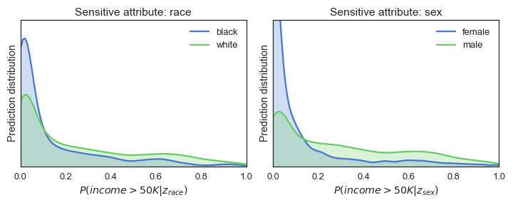
Are our results similar to those of our earlier blog using keras and TensorFlow? Pretty much! The ROC AUC, accuracy and probability distributions look very similar.

Unfortunately, switching frameworks did not magically make the classifier fairer. We can see this from the probability p%-rule and distributions, but also from the ROC AUC score of the adversary. A score higher than 0.5 indicates that the adversary is able to detect unfairness.
Training for fairness
Now that we have an unfair classifier and an adversary that is able to pick up on unfairness, we can engage them in the zero-sum game to make the classifier fair. Remember that the fair classifier will be punished according to:
\min_{\theta_{clf}}\left[Loss_{y}(\theta_{clf})-\lambda Loss_{Z}(\theta_{clf},\theta_{adv})\right].The first term represents how good the classifier is in predicting income, the second how good the adversary can reconstruct unfairness. The parameter \lambda represents the trade-off between these terms: it weighs the punishment by the adversary versus the prediction performance.
The adversary learns on the full data set and the classifier is given only the single batch, giving the adversary a slight edge in learning. The loss function for the classifier is changed to its original loss plus the weighted negative adversarial loss.
N_EPOCH_COMBINED = 165

for epoch in range(1, N_EPOCH_COMBINED):

    # Train adversary
    for x, y, z in data_loader:
        adv.zero_grad()
        p_y = clf(x)
        p_z = adv(p_y)
        loss_adv = (adv_criterion(p_z, z) * lambdas).mean()
        loss_adv.backward()
        adv_optimizer.step()

    # Train classifier on single batch
    for x, y, z in data_loader:
        pass  # Ugly way to get a single batch
    clf.zero_grad()
    p_y = clf(x)
    p_z = adv(p_y)
    loss_adv = (adv_criterion(p_z, z) * lambdas).mean()
    clf_loss = clf_criterion(p_y, y) - (adv_criterion(adv(p_y), z) * lambdas).mean()
    clf_loss.backward()
    clf_optimizer.step()
Conclusion
This blog took you through the steps of implementing a fair classifier in PyTorch. You can find this and the original keras implementation in our GitHub repo. Please consider opening a Pull Request if you’ve succesfully applied this model to your dataset!
Props to Stijn for the original implementation and reviewing this blog!
Improve your Python skills, learn from the experts!
At GoDataDriven we offer a host of Python courses taught by the very best professionals in the field. Join us and level up your Python game:
- Data Science with Python Foundation – Want to make the step up from data analysis and visualization to true data science? This is the right course.
- Advanced Data Science with Python – Learn to productionize your models like a pro and use Python for machine learning.


