7 Practical Tips for Demand Forecasting: Experimentation and Modeling

Demand forecasting appears straightforward: use historical data to fit a model, then use that model to predict what happens next. In practice, much of the difficulty lies in the decisions surrounding the model, which determine whether promising results in a notebook will hold up in production.

I recently encountered many of these decisions during a demand forecasting project in the energy sector. The project reinforced lessons from earlier forecasting work and surfaced several new ones, most of which extend well beyond this particular domain. The same principles apply to retail demand, logistics volumes, and other time-varying quantities. For a broader perspective on the strategic choices involved, including whether to buy or build a forecasting solution, see Demand Forecasting: Buy or Build?.

This is the first article in a two-part series and focuses on the experimentation and modeling phase. The follow-up will examine what happens beyond the notebook, covering the practical work required to bring a forecasting model into production.

Guard against data leakage from the start

Data leakage is one of the most important issues to address early, as it can make a model appear far more accurate than it will be in production. Leakage occurs when information that would not be available at prediction time enters the training data, creating an unrealistic evaluation that often becomes apparent only after deployment.

A common source of leakage in forecasting is the random train-test split. Shuffling observations and reserving 20% for testing is standard practice in many machine learning problems, but it breaks the temporal structure of forecasting data. As a result, patterns from the future can influence a prediction that should rely only on information available at that point in time, making the performance estimate unreliable.

The appropriate alternative is walk-forward validation, also known as expanding-window or time series cross-validation. The model is first trained on an initial block of historical data and evaluated on the period immediately following it. The cutoff is then moved forward, newly available observations are added to the training data, and the model predicts the next period. Repeating this process ensures that every evaluation reflects how the model will operate in production.

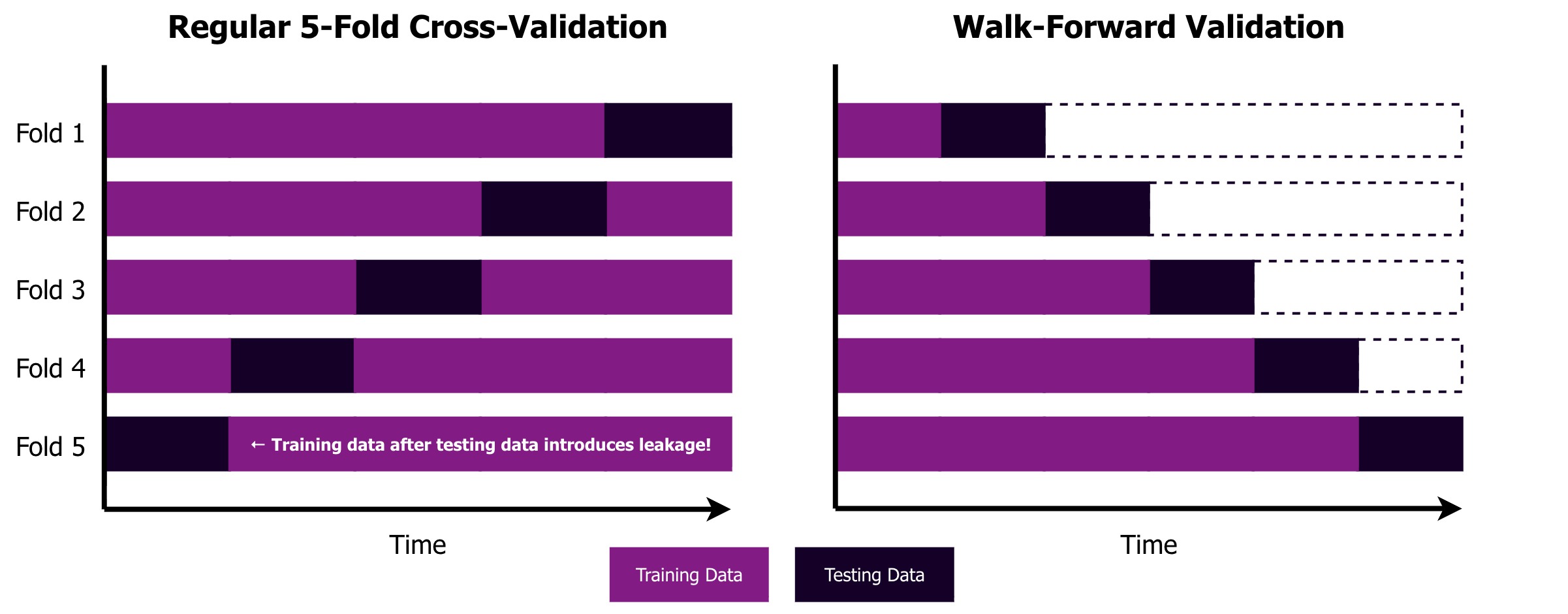
A time-aware split alone does not prevent leakage from entering through the features themselves. Rolling averages, for example, must be calculated using only values available before the prediction is made, rather than accidentally incorporating observations from the forecast period.

Other features require distinguishing between historical values and the information that will be available during the forecast period. For example, historical weather observations may be available for training, but future conditions should be represented by a weather forecast rather than the weather that was eventually observed. This is usually a reasonable approach, but keep in mind that a systematic difference between observed and forecasted covariates can reduce accuracy. By contrast, appointments or bookings scheduled in advance may already be known across the entire forecast horizon and can therefore be used without introducing leakage.

A practical way to assess this is to examine each feature at the boundary between the training period and the forecast period. Determine whether future values are known in advance, require a realistic proxy such as a weather forecast, or are unavailable and should therefore be excluded. Applying the same rules during validation prevents future information from entering the evaluation and provides a more credible estimate of production performance.

Choose metrics that reflect business costs

Standard regression metrics such as RMSE and MAE measure how far predictions deviate from reality. They are useful for comparing models, but they do not show what forecast errors actually cost the business. A 10% reduction in RMSE may look impressive on paper, but without understanding the operational impact, it is difficult to judge whether that improvement justifies a month of engineering effort.

A practical way to close this gap is to define a business cost metric alongside statistical metrics. Rather than measuring only the size of forecast errors, this metric estimates their financial or operational consequences. The exact formulation depends on the domain and should be developed with the stakeholders who experience those consequences, ensuring that model evaluation reflects the decisions the forecast is intended to support.

This distinction matters because forecast errors rarely have the same consequences in both directions. Overpredicting demand may result in excess inventory, unused capacity, or unnecessary procurement, while underpredicting may lead to missed contractual obligations, expensive emergency purchases, or lost revenue. Standard metrics treat both errors as equivalent, whereas a business cost metric can capture the asymmetry by assigning different penalties to each outcome.

This does not mean statistical metrics should be discarded, as they remain valuable for measuring predictive quality in a consistent and objective way. Business cost metrics complement them by expressing performance in terms stakeholders care about: reporting that a model change reduced expected operational costs by €50,000 per month often provides a stronger basis for investment than reporting a small reduction in RMSE alone.

Start with a proper baseline

When building a forecasting model, it is tempting to reach for gradient boosting or deep learning architectures right away. A better approach is to start with the simplest method that could work, then add complexity only when the results justify it. The first step is therefore to establish a baseline that sets a minimum level of performance for more advanced models to improve upon.

In forecasting, this baseline can take several forms. For example, a naive baseline may simply carry the last observed value forward, while a seasonal naive baseline uses the last value from the corresponding period. Linear regression on a handful of obvious features, such as the time of day, the day of the week, and recent lags, can also add some sophistication without introducing much complexity.

These simple models establish what can be achieved using basic temporal patterns. If a carefully tuned XGBoost model outperforms a naive baseline by only 2%, the additional complexity may not justify the maintenance cost, debugging difficulty, and operational risk it introduces.

Baselines also remain useful in production, where they can serve as fallback models and provide a sanity check when the primary model produces an implausible forecast. The principle is to increase complexity incrementally, allowing each step to earn its place through improvements in predictive accuracy or business value that outweigh the additional maintenance burden.

Distinguish between demand and observed outcomes

The target a forecasting model should learn is not always the variable recorded in the training data. Sales, consumption, and fulfilled orders represent observed outcomes, but operational constraints can prevent them from reflecting the underlying demand accurately.

The classic retail example is a product that goes out of stock. Sales fall to zero because no more units can be sold, not because customers have stopped wanting the product. Training directly on those observations teaches the model that demand disappeared during the stockout. Similar censoring occurs in other domains due to various operational constraints.

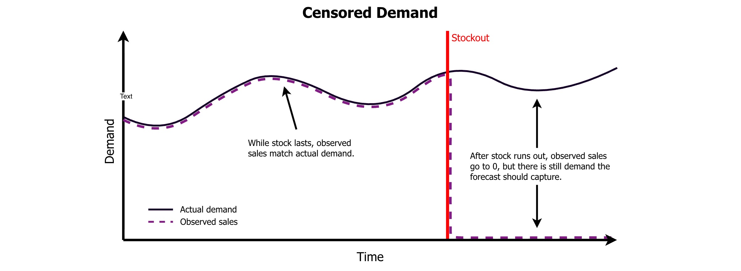
When constrained periods can be identified, a rough correction may already improve the target. Demand could be imputed from recent trends, while auxiliary signals such as search queries, attempted orders, or capacity utilization may provide additional evidence of unmet demand. When stockouts are rare, excluding those periods may be a practical alternative. However, be aware that this can cause underprediction, as stockouts often occur when demand is high. The right approach is naturally domain-specific and depends on whether a more accurate target justifies the added complexity.

The important step is to recognize the distinction and make a deliberate choice. Using the observed outcome may be sufficient for a particular use case, but it should not become the prediction target simply because it is the most convenient variable available.

Align the model with business context

Once the prediction target is clear, the downstream process that uses the forecast should determine what form it takes. Planning, scheduling, and procurement processes operate at specific levels of granularity, and the model should be designed around the information those processes require.

A common mistake is to model at a finer resolution than the decision requires. Hourly data may be available, but if the forecast is consumed only as a daily or weekly total, modeling every hour introduces additional noise, computation, and complexity without necessarily improving the decision. Matching the prediction granularity to the decision granularity keeps the model focused on the problem it needs to solve.

Business context should also guide feature engineering. Calendar variables such as the day of the week, the month, and public holidays provide an obvious starting point, while domain-specific events such as maintenance windows, seasonal transitions, and contractual periods may explain patterns that generic time features cannot capture.

Known constraints on the output deserve the same attention. If forecasts cannot be negative or must remain within operational limits, those requirements can be incorporated through the loss function, post-processing, or simple clipping. Encoding such constraints prevents the model from producing predictions that may be statistically plausible but practically impossible.

Track experiments systematically

Once experimentation begins, the number of possible configurations grows quickly as features, model architectures, and hyperparameters get added. Without a systematic record, it becomes difficult to compare results or determine which combination of code and settings produced a particular outcome.

Adopt MLflow, or a similar experiment tracking tool, early in the project. Logging the parameters, metrics, and artifacts for every run creates a searchable history of what was tried and makes meaningful comparisons possible as the number of experiments grows.

One specific recommendation is to log the Git commit hash alongside each experiment, as settings alone do not identify the code that produced the result. Together, the tracked parameters and commit hash provide a reliable link between an experiment, its configuration, and the exact implementation that was evaluated.

Invest in configuration management

Experiment tracking is only useful when the settings for each run are captured consistently. Data paths, feature toggles, hyperparameters, training windows, and forecast horizons often begin as hardcoded values or scattered command-line flags, but this approach becomes difficult to manage as the project grows.

A lightweight solution is to define a configuration dataclass from the start and use a library like pydargs to expose it through the command line. The dataclass then serves as both the configuration object used by the code and the source of the command-line interface, keeping both representations synchronized. A previous blog post covers pydargs in more detail.

from dataclasses import dataclass
from pydargs import parse

@dataclass
class ForecastConfig:
    """Forecasting pipeline configuration (will be logged to MLflow)."""

    model: str = "xgboost"
    lookback_days: int = 90
    include_weather: bool = True
    include_holidays: bool = True

config = parse(ForecastConfig)

Logging this configuration to MLflow alongside the Git commit hash records both the settings and the code behind every experiment. This makes successful runs easier to reproduce without adding much overhead to the development workflow.

Wrap-up

The lessons in this article deliberately focus on the foundations surrounding the model rather than on model architecture itself. Whether you choose XGBoost, an LSTM, a linear model, or a transformer certainly matters, but architecture is rarely the only factor limiting a forecasting project. A sophisticated model cannot compensate for leaked evaluation, a poorly defined target, a weak baseline, or metrics that are disconnected from business value, nor can it be improved systematically when experiments are difficult to reproduce.

Addressing these foundations makes model performance more credible and gives additional complexity a meaningful standard to beat. The follow-up article will move from experimentation to production, covering the serving infrastructure, monitoring, and operational practices required to keep a forecasting model reliable and useful over time.