The Linear Algebra Behind Linear Regression

Linear algebra is a branch in mathematics that deals with matrices and vectors. From linear regression to the latest-and-greatest in deep learning: they all rely on linear algebra “under the hood”. In this blog post, I explain how linear regression can be interpreted geometrically through linear algebra.

This blog is based on the talk A Primer (or Refresher) on Linear Algebra for Data Science that I gave at PyData London 2019.

Linear regression primer

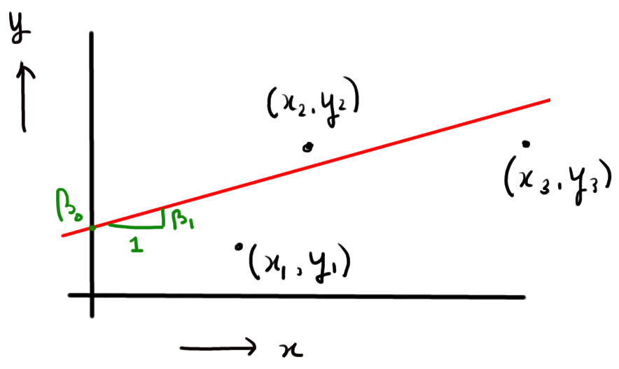
In Ordinary Least Squares (i.e., plain vanilla linear regression), the goal is to fit a linear model to the data you observe. That is, when we observe outcomes y_i and explanatory variables x_i, we fit the function

y_i = beta_0 + beta_1 x_i + e_i,

which is illustrated below

This boils down to finding estimators hat{beta}_0 and hat{beta}_1 that minimize the mean squared error of the model:

 min_{hat{beta}_0, hat{beta}_1}sum_{i=1}^n left( y_i - left( hat{beta}_0 + hat{beta}_1 x_i right) right)^2,

where n is the number of observations.

To solve this minimization problem, one way forward would be to minimize the loss function numerically (e.g., by using scipy.optimize.minimize). In this blog post, we take an alternative approach and rely on linear algebra to find the best parameter estimates. This linear algebra approach to linear regression is also what is used under the hood when you call sklearn.linear_model.LinearRegression.¹

Linear regression in matrix form

Assuming for convenience that we have three observations (i.e., n=3), we write the linear regression model in matrix form as follows:

underbrace{begin{bmatrix} y_1 \ y_2 \ y_3 end{bmatrix}}_{y} =
underbrace{begin{bmatrix} 1 & x_1 \ 1 & x_2 \ 1 & x_3 end{bmatrix}}_{X}  underbrace{begin{bmatrix}beta_0 \ beta_1 end{bmatrix}}_{beta} + underbrace{begin{bmatrix} e_1 \ e_2 \  e_3 end{bmatrix}}_{e} = Xbeta + e

Note that the matrix-vector multiplication Xbeta results in

 X beta = begin{bmatrix} beta_0 + beta_1 x_1 \ beta_0 + beta_1 x_2 \ beta_0 + beta_1 x_3 end{bmatrix},

which is essentially just a compact way of writing the regression model.

Geometrical representation of least squares regression

The objective is to obtain an estimator hat{beta} such that y approx Xhat{beta} (note that, usually, there is no hat{beta} such that y = Xhat{beta}; this only happens in situations that are unlikely to occur in practice).

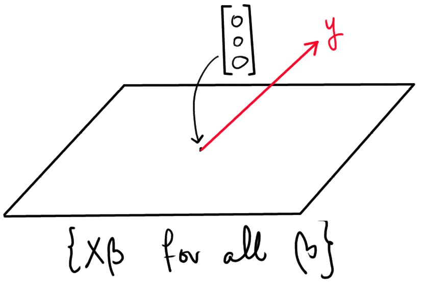
To represent the problem of estimating hat{beta} geometrically, observe that the set

 { Xhat{beta} text{ for all possible } hat{beta} }

represents all the possible estimators for hat{y}. Now, imagine this set to be a plane in 3D space (think of it is a piece of paper that you hold in front of you). Note that y does not "live" in this plane, since that would imply there is a hat{beta} such that Xhat{beta} = y. All in all, we can represent the situation as follows:

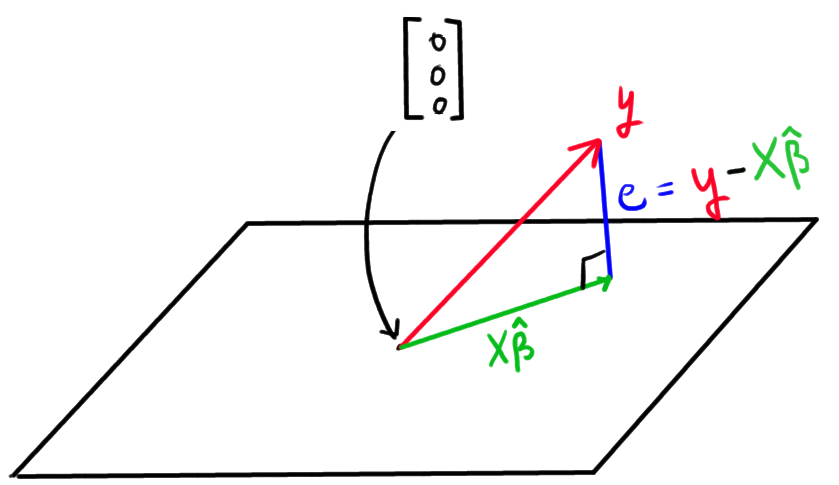
Finding the best estimator hat{beta}, now boils down to finding the point in the plane that is closest to y. Mathematically, this point corresponds with the hat{beta} such that the distance between Xhat{beta} and y is minimized. In the following figure, this point point is represented by the green arc:

Namely, this is the point in the plane such that the error (e) is perpendicular to the plane. It is interesting to note that minimizing the distance between Xhat{beta} and y means minimizing the norm of e (vector norms are used in linear algebra to give meaning to the notion of distance in higher dimensions than two):

 text{"norm of $e$"} = | e | = | y - Xhat{beta} | = sum_{i=1}^n left(y_i - left( hat{beta}_0 + hat{beta}_1 x_i right)right)^2, 

hence we are minimizing the mean squared error of the regression model!

Estimating the ß's

It remains to find a hat{beta} such that the vector e=y-Xhat{beta} is perpendicular to the plane. Or, in linear algebra terminology: we are looking for the hat{beta} such that e is orthogonal to the span of X (orthogonality generalizes the notion of perpendicularity to higher dimensions).

In general, it holds that two vectors u anv v are orthogonal if u^top v = u_1v_1 + ... + u_n v_n = 0 (for example: u=(1,2) and v=(2, -1) are orthogonal). In this particular case, e is orthogonal to X if e is orthogonal to each of the columns of X. This translates to the following condition:

(y-Xhat{beta})^top X =0.

By applying some linear algebra tricks (matrix multiplications and inversions), we find that:

X^top left(y - Xhat{beta}right) = 0 Leftrightarrow\
X^top y -  X^top Xhat{beta}  = 0 Leftrightarrow \
X^top y = X^top Xhat{beta} Leftrightarrow \
left( X^top Xright)^{-1} X^top y = hat{beta} 

Hence, hat{beta} = left( X^top Xright)^{-1} X^top y is the estimator we are after.

Numerical example

Suppose we observe:

x = [1, 1.5, 6, 2, 3]
y = [4, 7, 12, 8, 7]

Then, to apply the results from this blog post, we first construct the matrix X:

X = np.asarray([np.ones(5), x]).T
print(X)
>>> [[1.  1. ]
>>>  [1.  1.5]
>>>  [1.  6. ]
>>>  [1.  2. ]
>>>  [1.  3. ]]

and then do the matrix computations²

from numpy.linalg import inv
beta_0, beta_1 = inv(X.T @ X) @ X.T @ y
print(beta_0, beta_1)
>>> (4.028481012658229, 1.3227848101265818)

which gives us our esimates. To illustrate these, results

x_lin_space = np.linspace(0, 7, 100)
y_hat = beta_0 + beta_1 * x_lin_space
plt.scatter(x, y, marker='x')
plt.plot(x_lin_space, y_hat, color='r')

which shows the fit of our model:

Although this blog post was written around a simple example with only one feature, all the results generalize without any difficulties to higher dimensions (i.e., more observations and more features).

If you have enjoyed this post, probably the fast.ai course on computational linear algebra is for you (it's free).

Improve your Python skills, learn from the experts!

At GoDataDriven we offer a host of Python courses taught by the very best professionals in the field. Join us and level up your Python game:

• Data Science with Python Foundation - Want to make the step up from data analysis and visualization to true data science? This is the right course.
• Advanced Data Science with Python - Learn to productionize your models like a pro and use Python for machine learning.