With deep learning applications blossoming, it is important to understand what makes these models tick. Here I demonstrate, using simple and reproducible examples, how and why deep neural networks can be easily fooled. I also discuss potential solutions.

Several studies have been published on how to fool a deep neural network (DNN). The most famous study, which was published in 2015 used evolutionary
algorithms or gradient ascent to produce the adversarial images.1 A very recent study (October 2017) revealed that fooling a DNN could be achieved by changing a single pixel.2 This subject seems fun and all but has substantial implications on current and future applications of deep learning. I believe that understanding what makes these models tick is extremely important to be able to develop robust deep learning applications (and avoid another event like random forest mania).3
A comprehensive and complete summary can be found in the When DNNs go wrong blog, which I recommend you to read.
All these amazing studies use state of the art deep learning techniques, which makes them (in my opinion) difficult to reproduce and to answer questions we might have as non-experts in this subject.
My intention in this blog is to bring the main concepts down to earth, to an easily reproducible setting where they are clear and actually visible. In addition, I hope this short blog can provide a better understanding of the limitations of discriminative models in general. The complete code used in this blog post can be found here.
Discriminative what?
Neural networks belong to the family of discriminative models, they model the dependence of an unobserved variable (target) based on observed input (features). In the language of probability this scenario is represented by the conditional probability and it is expressed as:
p(target|features)it reads: the probability of the target given the features (e.g. the probability that it will rain based on yesterday’s weather, temperature and pressure measurements).
Multinomial logistic regression models are also part of these discriminative models and they basically are a neural network without a hidden layer. Please don’t be disappointed but I will start by demonstrating some concepts using multinomial logistic regression. Then I’ll expand the concepts to a deep neural network.
Fooling multinomial logistic regression
As mentioned before a multinomial logistic regression can be seen as a neural network without a hidden layer. It models the probability of the target (Y) being a certain category (c), as a function (F) that depends on the linear combination of the features ()). We write this as
P(Y=c|X)=F(\theta_{c}^T\cdot X)where $\theta_c$ are the coefficients of the linear combination for each category. The predicted class by the model is the one which gives the highest probability.
When the target Y is binary, F is taken to be some sigmoid function, the most common being the logistic function. When Y is multiclass we commonly use F as the softmax function.
Apart from the conceptual understanding of discriminative models, the linear combination of the features ($\theta_{c}^T\cdot X$) is what makes classification models vulnerable as I will demonstrate. In the own words of Master Jedi Goodfellow: "Linear behavior in high-dimensional spaces is sufficient to cause adversarial examples".4
Iris dataset
When I was thinking on how to do this blog post and actually visualize the concepts, I concluded I needed two things:
- A 2-dimensional feature space.
- A model with high accuracy on this space.
The 2-dimensional space because I wanted to generate plots which directly show the concepts. High accuracy because it’s meaningless if I am able to fool a bad model.
Lucky for me, it turns out that a good accuracy can be obtained on the Iris dataset by just keeping two features: petal length and petal width.
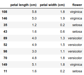
Putting everything into shape this is how the data looks like

This dataset contains only 150 observations, I will fit the model to all the data using a cross-entropy loss function and a L2 regularization term. This is just a plug and play from the amazing scikit-learn.
model = LogisticRegression(max_iter=100, solver='lbfgs', multi_class='multinomial', penalty='l2')
model.fit(X=iris.loc[:, iris.columns != 'flower'], y=iris.flower)
The mean accuracy of the model is $96.6\%$. This score is based on the training data and can be misleading, even if I am using a regularization term I can still be overfitting.5
Let’s now look at our predictions and at how our model is drawing the classification boundaries.

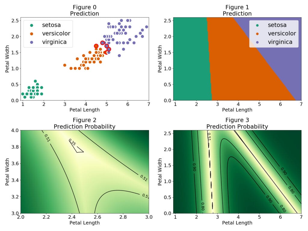
In Figure 0 the red outer circles indicate those observations that were wrongly classified. The setosa flowers are easily identified and there is a region where the versicolor and virginica observations are close together. In Figure 1 we can see the different regions for each flower category. The regions are separated by a linear boundary, this is a consequence of the linear combination model used $P(Y=c|X)=F(\theta_{c}^T\cdot X)F$ is the logistic function
F(\theta_{c}^T\cdot X)=\frac{1}{1 + e^{-\theta_{c}^T\cdot X}}and the classification boundary is given by P(Y=c|X)=\frac{1}{2} \theta_{c}^T\cdot X=0. If the features are in one dimension then the boundary will be a single value, for two features the boundary is a single line and for three features a plane and so on. In our multinomial case we use the softmax function
F(\theta_{c}^T\cdot X)=\frac{e^{\theta_{c}^T\cdot X}}{\Sigma_{i=1}^Ne^{\theta_{i}^T\cdot X}}where the sum over i in the denominator runs over all the possible classes of the target. In the regions where only two classes have a non-negligible probability the softmax function simplifies to the logistic function. Therefore the linear classification boundaries between two regions is given by the contour P(Y=c|X)=\frac{1}{2} P(Y=c|X)=\frac{1}{3} where the uncertainty of our prediction is maximum. This region is illustrated in Figure 2.
A thing to note is that the regions extend to values which can be very far from the observations, which means we can grab a petal length of 1 and petal width of 4 and still be classified as a setosa. Even more, Figure 4 shows that even far away from our observations we can find regions with extremely high probability. We can even use a negative petal length!

Let’s pick some points from Figure 4 and see if I am able to fool the multinomial logistic classifier:
- Point: (.1, 5)
- Prediction: setosa
- Probability: 0.998
- Point: (10, 10)
- Prediction: virginica
- Probability: 1.0
- Point: (5, -5)
- Prediction: versicolor
- Probability: 0.992
Go hands-on with deep learning yourself!
Join us for a three-day course on Deep Learning. The course starts with an introduction into the backgrounds of deep learning and ends with you building your own deep learning application. It’s great for data scientists that have experience with Python and work with unstructured data, like text, images and speech.


