Neural networks are everywhere nowadays. But while it seems that
literally everyone is using a neural network today, creating and
training your own neural network for the first time can be quite
a hurdle to overcome. In this blog post I’ll take you by the hand
and show you how to train an image classifier — using PyTorch!
Why not Keras?
Before we start, you might ask why I’ve chosen to use PyTorch,
and not Keras. Of course there are pros and cons for each of the
options, but I am not going to attempt to make a good overview here.
I’m not the right person to ask for a comparison because I
have no experience with Keras, so if you are looking for an article
on the differences between these (and possibly more) options
you could have a look here,
here
or here.
Convolutional Neural Networks
The tool that we are going to use to make a classifier is called a
convolutional neural network, or CNN. You can find a great explanation
of what these are right
here on wikipedia.
But we are not going to fully train one ourselves: that would take way more time
than I would be willing to spend. Instead, we are going to do transfer learning,
where we take a pre-trained CNN and replace only the last layer by a layer
of our own. Then we only need to train that single layer, as all the other
layers already have weights that are quite sensible. Here we exploit the fact
that the images we are interested in have a lot of the same properties
as those images that the original network was trained on. You can find a
great explanation of transfer learning
here.
Defining a neural network
Before we do any transfer learning, lets have a look at how we can define
our own CNN in PyTorch. Here is a minimal example:
from torch.nn import Conv2d, functional as F, Linear, MaxPool2d, Module

class Net(Module):

    def __init__(self):
        super(Net, self).__init__()
        self.conv = Conv2d(3, 18, kernel_size=3, stride=1, padding=1)
        self.pool = MaxPool2d(kernel_size=2, stride=2, padding=0)
        self.fc1 = Linear(18 * 16 * 16, 64)
        self.fc2 = Linear(64, 10)

    def forward(self, x):
        x = F.relu(self.conv(x))
        x = self.pool(x)
        x = x.view(-1, 18 * 16 * 16)
        x = F.relu(self.fc1(x))
        x = self.fc2(x)
        return x
We define a neural network by creating a class that inherits from Module.
When we initialise the network we define the layers of the network:
- a 2D convolutional layer,
- a max pooling layer,
- two linear layers.
In the forward method we define what happens to any input x that we feed
into the network. This argument x is a PyTorch tensor (a multi-dimensional
array), which in our case is a batch of images that each
have 3 channels (RGB) and are 32 by 32 pixels: the shape of x is then (b, 3, 32, 32)
where b is the batch size.
The first statement of our forward method applies the convolutional layer
to the input, which results in a 18-channel, 32 by 32 tensor for each input image.
Immediately after that we apply
the ReLU function.
Next, we apply the max pooling layer, which reduces the tensor to size (b, 18, 16, 16).
The view method of x reshapes the tensor to the specified shape, where the
value of -1 indicates that PyTorch is supposed to figure out this dimension: this
allows us to work with varying batch sizes. The result is a 1D vector of size 4608
for each element of our batch.
Finally, we apply the two linear (fully connected) layers with yet another
relu in between. This first reduces our shape from (b, 4608) to (b, 64) and then
to (b, 10): our output is 10 values for each image.
We can interpret these outputs as the some kind of probability for each
class to be the correct class: this model would be a classifier for 10 classes.
Using a pre-trained model
If instead of defining our own model we want to use a pre-trained model,
PyTorch provides quite a few that we can easily use. All we need to do to use
Squeezenet for example is:
from torchvision.models import squeezenet1_0

model = squeezenet1_0(pretrained=True)
We can have a look at the structure of this model by simply printing it:
print(model) gives us:
SqueezeNet(
  (features): Sequential(
    (0): Conv2d(3, 96, kernel_size=(7, 7), stride=(2, 2))
    (1): ReLU(inplace)
    (2): MaxPool2d(kernel_size=3, stride=2, padding=0, dilation=1, ceil_mode=True)
    (3): Fire(
      (squeeze): Conv2d(96, 16, kernel_size=(1, 1), stride=(1, 1))
      (squeeze_activation): ReLU(inplace)
      (expand1x1): Conv2d(16, 64, kernel_size=(1, 1), stride=(1, 1))
      (expand1x1_activation): ReLU(inplace)
      (expand3x3): Conv2d(16, 64, kernel_size=(3, 3), stride=(1, 1), padding=(1, 1))
      (expand3x3_activation): ReLU(inplace)
    )
    ...
  )
  (classifier): Sequential(
    (0): Dropout(p=0.5)
    (1): Conv2d(512, 1000, kernel_size=(1, 1), stride=(1, 1))
    (2): ReLU(inplace)
    (3): AvgPool2d(kernel_size=13, stride=1, padding=0)
  )
)
The network consists of two parts: the features and the classifier.
I’ve truncated the output of the features part in order to keep some
readability: it contains 12 layers out of which eight are Fire modules.
These modules contain six sublayers and are the defining feature of Squeezenet,
read more about them here.
For us the classifier part is much more interesting though: this is where
the network makes the final classification based on the features that were
created in the previous layers. If we want to do transfer learning, this
is the layer that we want to replace.
Note that Squeezenet was designed for and trained upon an
ImageNet
data set, which contains 1000 classes. We can replace the Conv2d layer
with our own layer with the appropriate number of classes. For example:
model.num_classes = n_classes
model.classifier[1] = nn.Conv2d(512, n_classes, kernel_size=(1, 1), stride=(1, 1))
Here we also set the num_classes attribute of the network which is internally
used to re-shape the final output of the network.
Training
Now that we have a model set up, the next step is training it. For that
we need the following train loop:
from torch.nn import CrossEntropyLoss
from torch.optim import SGD

model.train()

criterion = CrossEntropyLoss()
optimizer = SGD(model.parameters(), lr=1E-3, momentum=0.9)

for inputs, labels in loader:
    optimizer.zero_grad()
    outputs = model(inputs)

    loss = criterion(outputs, labels)

    loss.backward()
    optimizer.step()
First, we set the model to training mode — I’ll explain below what that means.
Next, we define our loss,
Cross-Entropy loss, and our optimizer:
Stochastic Gradient Descent.
Let’s not worry about the parameters of the optimizer just yet.
The we start the training loop. We loop over the contents of a loader object,
which we’ll look at in a minute. Every iteration it yields two items:
the inputs and the labels. They are PyTorch tensors of which the
first dimension is the batch size. The inputs can be
directly fed to the model, while labels has the single dimension of which
the size is equal to the batch size: it represents the class of each image.
We start each iteration by resetting the optimizer by calling zero_grad,
and then feeding the inputs through the model. Next, we use our loss function
to compute the loss on the results of the model. While we do those computations
PyTorch automatically tracks our operations and when we call backward() on
the result it calculates the derivative (gradient) of each of the steps
with respect to the inputs. This gradient is then what the optimizer can
use to optimize the weights when we call step().
We call the full training loop over all elements in the loader an epoch.
Evaluation
After training for one or more epochs you are probably interested in the
performance of your network. We can evaluate that by computing the total
loss on the evaluation set, like this:
from torch import max, no_grad

model.eval()

loss = 0
with no_grad():
    for inputs, labels in loader:
        outputs = model(inputs)
        loss += criterion(outputs, labels)
        _, predictions = max(outputs.data, dim=1)
        ...
First we need to set our model to evaluation mode (which is the same
as disabling the training mode using .train(False)). This disables features
that are handy using train time, such as
dropout, in
order to get the maximum performance out of our network. Next, we enter the
no_grad context, in which the automatic computation of gradients is disabled:
we do not need that during evaluation.
Then we have a loop similar to the one in the training case: we loop over
the inputs and the labels from the loader, pass the inputs to the model
and calculate the loss. In addition, we could inspect the predictions of the
model (and possibly use them) by using the torch.max function, which returns
a tuple of (maximum values, positions). These positions correspond to the output
node (and hence class) that has the highest probability according to our model,
which we can interpret as the index of the most probable class.
The loader
Of course data is essential to either training or evaluating a classifier.
In the previous two segments we looped through the contents of this loader
object, which we did not define before. In order to create it, we must first
define a data set.
Of course a single data set is not enough: we need both a training and a testing
data set. In addition you may want to have a validation data set as well.
Assuming that you have your images in a folder structure like this:
images/
  train/
    class_1/
    class_2/
    ...
  train/
    class_1/
    class_2/
    ...
we can define the data sets as follows:
from torchvision import transforms
from torchvision.datasets import ImageFolder

train_transform = transforms.Compose([
    transforms.RandomResizedCrop(224),
    transforms.RandomHorizontalFlip(),
    transforms.ToTensor(),
])
test_transform = transforms.Compose([
    transforms.Resize(256),
    transforms.CenterCrop(224),
    transforms.ToTensor()
])

train_set = ImageFolder('images/train', transform=train_transform)
test_set = ImageFolder('images/test', transform=test_transform)
To each image set we provide a transformation which tells PyTorch what to
do with the images when reading them. We define two transformations,
one for each data set.
Let’s have a look at the test_transform first: when we read a test image, we
- resize the image such that the smallest dimension of the image is 256 pixels, then we
- crop a square of 224 x 224 pixels from the center of the resized image, and finally
- convert the result to a tensor so that PyTorch can pass it through a model.
In the train_transform we do something different: we
- randomly take a crop of a random size (between certain limits) and aspect ratio and resize that to 224×224,
- randomly flip the image horizontally, and finally
- convert the result to a tensor.
This means that although the model will encounter each training image once during
every epoch, the exact images it will be seeing vary from epoch to epoch: sometimes
it will be seeing most of the image and other times it will see only a small crop.
Since most objects still look roughly the same when we horizontally flip the image,
we want the model to also learn from the flipped images. Vertically flipped (upside-down)
images usually do not look like the same object anymore, so we only flip horizontally.
All this randomly transforming the training images helps to prevent our model
to overfit:
it cannot learn by heart that a small portion of an image belongs to a certain
label because every epoch it sees a different subset of the image.
Once we have defined the data sets, we can create the loaders:
from torch.utils.data import DataLoader

train_loader = DataLoader(
    dataset=train_set,
    batch_size=32,
    num_workers=4,
    shuffle=True,
)

test_loader = DataLoader(
    dataset=test_set,
    batch_size=32,
    num_workers=4,
    shuffle=True,
)
To each we provide the respective data set, and we specify that:
- the batch size is 32 (feel free to try other values),
- we want four processes to read and transform the images, and
- we want to read the images in random order.
Now we have all ingredients to really start training our model! But…
Learning rate
Back when we defined the optimizer,
optimizer = SGD(model.parameters(), lr=1E-3, momentum=0.9)
we skipped over its parameters. And especially the first one, lr, the learning rate,
is very important. This parameter defines how much the weights will be changed
in every optimization step. In other words, it defines our step size when we are
looking for the most optimal set of weights.
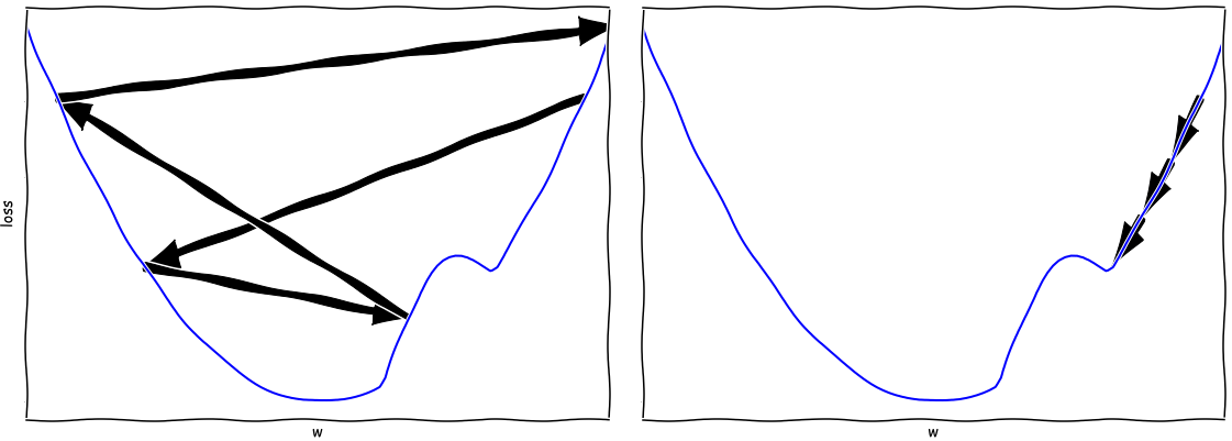
Let’s have a look at a 1D example. Suppose we are looking to find the minimum value
in the curves depicted below. If our learning rate is too large then we might
actually walk away from the minimum, as we see on the left. If, on the other hand
our learning rate is too low, we will be moving very slowly and we run the risk
of getting stuck in a local optimum.

Now you might be inclined to perform a classical hyper-parameter search, by simply
trying out a lot of values for the learning rate and seeing how well the model
performs in the end. But training a single
models takes at least a few hours on a decent GPU, so training tens (or hundreds!)
of these models would become a costly affair.
A better way to figure out the optimal value of the learning rate is to do a learning
rate sweep: we train our model for a number of batches for a range of learning
rates. In the example here I’ve included a little pseudocode:
def set_learning_rate(optimizer, learning_rate):
    for param_group in optimizer.param_groups:
        param_group['lr'] = learning_rate

learning_rates = np.logspace(min_lr, max_lr, num=n_steps)
results = []
for learning_rate in learning_rates:
    set_learning_rate(optimizer, learning_rate)
    train_batches(...)
    results.append(evaluate(...))
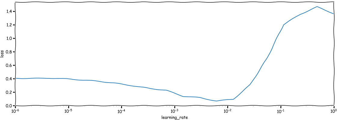
The result should look something like this:

We see that in the beginning we learn very very slowly, but it improves
after a while. Then, when the learning rate passes some point around (10^{-2}) we
see the performance of our network going down (the loss goes up), up to the
point where the results are terrible. Your ideal setting is there where the
improvement is the fastest, i.e. where the line goes down the steepest. For the above
example that would be somewhere around (10^{-3}).
After the sweep, do not forget to reset the network to the state before you did the sweep,
as the batches with the highest learning rates will most likely have ruined
your networks’ performance.
Learning rate scheduler
Unfortunately doing a sweep once is not enough, as the best learning rate depends on
the state of our network. The closer we come to the ideal weights, the lower we should
set our learning rate. We can solve this by using a learning rate scheduler.
For example, we can use the ReduceLROnPlateau scheduler which decreases the learning
rate when the loss has been stable for a while:
from torch.optim.lr_scheduler import ReduceLROnPlateau

scheduler = ReduceLROnPlateau(optimizer, factor=0.5, patience=10)
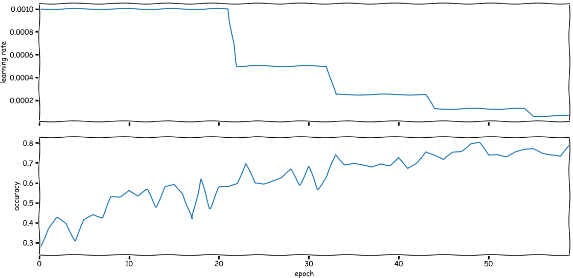
This scheduler is configured to reduce the learning rate by a factor 2 if the
performance was stable for 10 epochs.
All we have to do next is call scheduler.step(test_loss) after every epoch,
and the scheduler will automatically adapt the learning rate to the situation.
The result will look something like the figure below: every once in a while the scheduler
will decide to reduce the learning rate when it thinks the loss is not improving
enough.

Now all that you need to start making your own image classifier is a data set!
Where next?
If you’re looking for more example code, have a look at this project
which I used to build an image classifier that can recognize skylines of a few large cities.
I gave a talk about the project on EuroPython 2019, of which you can find the
slides here.
And of course the PyTorch docs are your
friend whenever you are building something like this!
Join us for more on deep learning!
Want to get the hang of deep learning? Our three-day Deep Learning course will take you through the theory you need to know and provides you with loads of hands-on experience.


