Part 1: from a business problem to a Bayesian solution
Bayesian modeling is a lesser known yet very promising area of Statistics and Data Science. It thrives where traditional approaches fail and comes with a few nice perks. In this series of blog posts we consider an illustrative business case about price optimization showing why Bayesian modeling and the related tech (such as the PyMC3 library for Python) is a useful set of tools to have in your data arsenal. We will learn how Bayesian modeling (unlike traditional approaches) allows us to skip determining arbitrary assumptions and thresholds, while transparently getting back not just point estimates but whole distributions of possible values.
The first part of this series will introduce you to an illustrative business case and the core Bayesian modeling concepts, translating the former into the language of the latter. The second part will focus on actually constructing Bayesian models (with PyMC3), making inferences and unleashing the full potential of the field. All data as well as all further analysis, graphs and models are available in this GitHub repository.
In principle, no prior knowledge of (Bayesian) Statistics is necessary, but having some would naturally simplify the read (see for example this series for some helpful prep material).
The business case
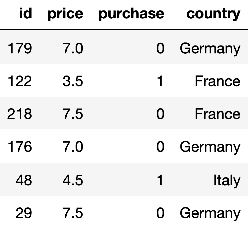
Consider a (fictional) B2B service provider company “Virtuoso” which operates in France, Germany, and Italy. Virtuoso can charge different prices in each country but does not know how to do so optimally. Their data consists of prices that have been offered historically in each country and led to a sale in some cases. Our goal will be to optimize their pricing strategy the Bayesian way. This will help Virtuoso not only to improve sales but to determine how distinct, price-sensitive, and uncertain each regional market is.

Understanding the problem
Before we continue, it is important to identify some potential issues in Virtuoso’s past operations and pricing strategy. This will aid us in formulating our data-driven solutions. From the data, we quickly identify that successful sales are not equally likely across all countries. Besides, for purchases made in each country sales prices also differ. Figure 1 illustrates these two observations for each country (using 95% confidence intervals to acknowledge data variability and potential data scarcity):

Why are more offers rejected in Germany than in Italy? The average purchasing price in Germany is lower, so customers might have tighter budgets and be more price-sensitive. Therefore, using the same pricing strategy in all countries might not be a good idea. Currently, proportional to the number of offers, revenues in Italy are more than twice as high as in Germany proportional to the number of offers. This clearly leaves some room for improvement. If we properly quantify price-sensitivity in each country, we could make such advances.
On the positive side, having data with both successful and unsuccessful offers in each country for various prices provides a perfect ground for using Bayesian analysis to understand between-country differences better and to develop more personalized sales strategies. Using the Bayesian approach we can not only make usual forecasts (that will help with suggesting better prices in each country), but also incorporate any insider perceptions about each country into the model (e.g. German budgets are more stringent). If these turn out somewhat wrong, the data will correct us. So, let’s get to it.
Theory in a nutshell
In essence, Bayesian modeling uses a form of Bayes Theorem to determine how the problem at hand really looks like given the observed data and our insider knowledge/believes. We may only have a rough idea about how fair a given coin is or how stringent German companies are, but with a bit of relevant data we can understand these problems much better. And Bayesian modeling tells us how exactly this new data should be considered in combination with our rough beliefs.
This approach presents several advantages: unlike traditional (frequentist) modeling approaches, there is less need to make questionable assumptions beforehand or to set and misuse arbitrary thresholds (p-values and such). Instead, we explicitly incorporate what we know about the problem beforehand (our priors). This is more intuitive, transparent and leaves less room for misinterpretation.

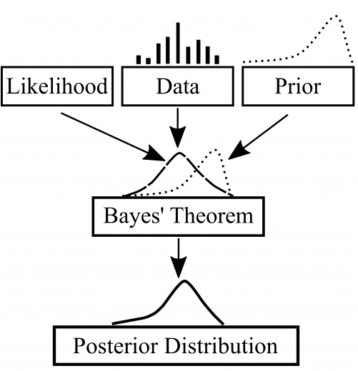
The rest is taken care of by Bayes Theorem. As a result, we acquire not just point estimates but distributions of possible model parameters with an indication of how much uncertainty there is about their values – a valuable quantification of how informative the observed data was (see Figure 2). This can in its turn translate into valuable business insights such as not just average predicted values, but a range of such values coupled with associated levels of certainty.

Engineering a Bayesian model
While helping Virtuoso, our goal is to apply Bayesian modeling such that we learn from the data about the relationship between prices and sales in each country. In Bayesian terms, we are after the posterior (post-learning) distributions of price sensitivity parameters (left part of Figure 3). As the Bayes formula for modeling in Figure 3 suggests, we need to determine three important parts.
- f(data|model) is the “likelihood distribution” – the statistical relationship that indicates how likely the data is, given our model. This component usually follows from the problem itself: many real life processes are binary events like coin flips, which is commonly modelled using a Bernoulli likelihood.
- f(model) is the “prior distribution” – another statistical relationship that acknowledges all initial information and believes that we have about the problem. If we have no such information, we deal with “uninformed priors”, indicating that everything is possible. If we have some domain knowledge, expectations or just pure intuition, this framework allows us to directly incorporate it here.
- f(data) is the most technical and least intuitive parameter. The good news is that it is basically a data-dependent constant value that can be ignored during practical modeling.
Bayes theorem tells us how to combine these three factors in a single equation that results in the posterior distribution. As a result, the observed data reshapes our prior distribution into a more informed one. In simpler terms, our initial understanding of what the problem entails mathematically evolves into a more informed one. Understanding this means understanding Bayesian modeling:

Translating the business case.
To conclude the first part of this series, let us translate the Virtuoso’s business case in the language of Bayes modeling. This will be essential to later construct and use actual models.
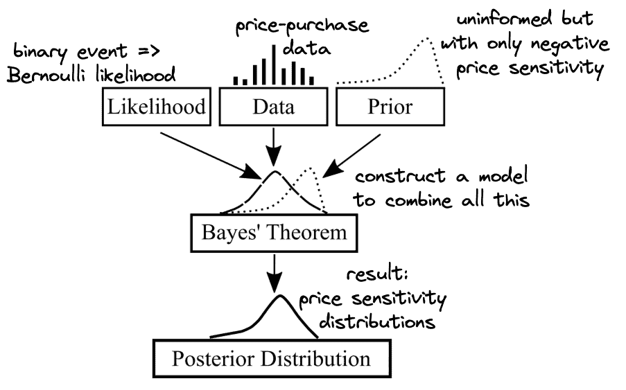
First, what are we actually after in this business case? We want to be better informed about purchasing behaviors across countries and differences in how price-sensitive clients are. Therefore, we are primarily after price sensitivity distributions (which may be different in each country). In Bayesian terms, we are attempting to acquire posteriors for price-sensitivity parameters – whole distributions, not just point estimates such as means. Once we have those, we will be able to compare international clients not just on average, but also in terms of risks and variation.
How will we acquire these posteriors? We are going to use Bayes formula together with the three core components introduced above.
Priors allows us to put any already available knowledge directly into the problem. For instance, as prices grow, customers are usually less willing to purchase. Consequently, our prior can capture that by restricting price sensitivities to only be of negative sign. Other than that, we may have little knowledge of what these parameters can possibly be. In such cases, an uninformed prior is commonly chosen to allow a broad range of possibilities.
Likelihood distribution concerns the process that turns our inputs (different prices) into some result (purchase or no purchase). This is a binary event, which in statistics is commonly modeled using Bernoulli distribution. There are many resources that help matching various real-life processes with appropriate statistical distributions.
Finally, using data in this framework comes naturally once everything else is defined. We already have data that matches price suggestions with the 0/1 result of purchase or no purchase. Such data is supplied to a Bayesian model that combines all its components to produce posterior distribution(s). However, actually doing this will have to wait until the next part of this series.
Short retrospective
So far in this first part of our series about doing business the Bayesian way, we identified a core analytical question from a realistic business case. Then we saw how it can be translated into the language of Bayesian modeling, while also getting introduced to some of the core concepts in this field. We can summarize our translation with the following illustration:

While we will hold on with constructing a model and analyzing the results until the next part, we can already appreciate some features of Bayesian modeling. This includes being able to include our prior knowledge directly into the problem, while allowing a possibility for it to be corrected if we are wrong. Every step is transparently modeled – which leaves less room for misinterpretation and hidden issues. Furthermore, thinking about the business problem in such structural terms helps to understand its essence. And in the end, we can anticipate not just a point estimate but broad information about the question at hand (involved risks, amount of uncertainty, variability etc.), which will be of higher value to the business.


