Artificial neural networks imitate concepts that we use when we think of the human brain. With Deep Learning, we can build such networks using large amounts of data to get models that outperform traditional models. This post demonstrates how neural networks leverage concepts like representation and memory.
We'll use embeddings and recurrent neural networks for sentiment classification of reviews from movies: we want to know if they contain a positive or negative sentiment. The code for this blog post is inspired by this keras example github.com/keras-team/keras/blob/master/examples/imdb_lstm.py. See the repository of our Code Breakfast if you'd like to play around with the code.
1 Data
Like many other libraries, keras includes some standard datasets to play around with.
We'll use the IMDB dataset.
This section shows what this dataset contains.
From the website (emphasis ours):
"Dataset of 25,000 movies reviews from IMDB, labeled by sentiment (positive/negative). Reviews have been preprocessed, and each review is encoded as a sequence of word indexes (integers). For convenience, words are indexed by overall frequency in the dataset, so that for instance the integer "3" encodes the 3rd most frequent word in the data. This allows for quick filtering operations such as: "only consider the top 10,000 most common words, but eliminate the top 20 most common words As a convention, "0" does not stand for a specific word, but instead is used to encode any unknown word.
We'll load reviews with only the 20,000 most frequent words:
from keras.datasets import imdb

NUM_WORDS = 20000

(x_train, y_train), (x_test, y_test) = imdb.load_data(num_words=NUM_WORDS)
x_train and x_test are numpy.ndarray' that contain list of sequences.
Two examples are show below: the samples don't have the same length and are encoded by integers.
> array([ list([1, 14, 22, 16, ..., 2]),
>       list([1, 194, 1153, 194, ..., 95])], dtype=object)
This may be a good way to represent text for machines, but it's not really useful for humans. The 'original' text may look something like this:
worst mistake of my life br br i picked this movie up at target for 5 because i figured hey it's sandler i can get some cheap laughs i was wrong completely wrong mid way through the film all three of my friends were asleep and i was still suffering worst plot worst script worst movie i have ever seen i wanted to hit my head up against a wall for an hour then i'd stop and you know why because it felt damn good upon bashing my head in i stuck that damn movie in the and watched it burn and that felt better than anything else i've ever done it took american psycho army of darkness and kill bill just to get over that crap i hate you sandler for actually going through with this and ruining a whole day of my life
Note the special words like
We need to do some more processing on the integer data: keras needs all sequences (or reviews) to be of equal length.
We can choose to pad all sequences to the longest length, or we can choose a maximum review length and cut longer reviews. We'll cut reviews after 80 words and pad them if needed:
from keras.preprocessing import sequence

MAXLEN = 80

X_train = sequence.pad_sequences(x_train, maxlen=MAXLEN)
X_test = sequence.pad_sequences(x_test, maxlen=MAXLEN)

X_train

> array([[   15,   256,     4, ...,    19,   178,    32],
>       [  125,    68,     2, ...,    16,   145,    95],
>       [  645,   662,     8, ...,     7,   129,   113],
>       ...,
>       [  529,   443, 17793, ...,     4,  3586,     2],
>       [  286,  1814,    23, ...,    12,     9,    23],
>       [   97,    90,    35, ...,   204,   131,     9]], dtype=int32)
Now that we have our data, let's discuss the concepts behind our model!
2 Model
Our model consists of three layers: an embedding layer, a recurrent layer and a dense layer. The embedding layer learns the relations between words, the recurrent layer learns what the document is about and the dense layer translates that to sentiment.
2.1 Embedding layer
The embedding layer embeds our original word vectors in a dense, lower-dimensional space. This embedding can capture complicated relationships between words and make it easier to learn.
We'll see in a minute what we mean with that, let's first start with the traditional approach of one-hot encoding. One-hot encoding words indexes words and represents them as a big vectors with zeros and ones.
With one-hot encoding, the vocabulary "(textsf{code - console - cry - cat - dog})" would be represented like this:
| has_code | has_console | has_cry | has_cat | has_dog | |
|---|---|---|---|---|---|
| code | 1 | 0 | 0 | 0 | 0 |
| console | 0 | 1 | 0 | 0 | 0 |
| cry | 0 | 0 | 1 | 0 | 0 |
| cat | 0 | 0 | 0 | 1 | 0 |
| dog | 0 | 0 | 0 | 0 | 1 |
The three text snippets "(textsf{code console})", "(textsf{cry cat})" and "(textsf{dog})" are represented by combining these word vectors:
| has_code | has_console | has_cry | has_cat | has_dog | |
|---|---|---|---|---|---|
| "code console" | 1 | 1 | 0 | 0 | 0 |
| "cry cat" | 0 | 0 | 1 | 1 | 0 |
| "dog" | 0 | 0 | 0 | 0 | 1 |
This representation has some problems.
This matrix will be very large for large vocabulary and also very empty. Many statistical models have problems learning from such big and sparse data. There are too many features to learn from and not enough samples to understand every feature. Combining words in an intelligent way could solve this.
In addition, treating words as atomic units throws away a lot of information. "(textsf{cat})" is more similar to "(textsf{dog})" than to "(textsf{code})", and "(textsf{console})" has a different meaning when occurring next to "(textsf{code})" than when it's next to "(textsf{cry})". These complex relationships cannot be represented by our simple one-hot encoding.
Instead of learning from one-hot encoding, we first let the neural network embed words in a smaller, continuous vector space where similar words are close to each other. The smaller space makes it easier to learn from and a continuous representation allows to learn complex relationships.
Such an embedding for our vocabulary could look like this:
| embedding_0 | embedding_1 | |
|---|---|---|
| code | 0 | 0.1 |
| console | 0.2 | 0.1 |
| cry | 0.5 | 0.4 |
| cat | 0.7 | 0.6 |
| dog | 0.8 | 0.7 |
We only need two dimensions for our words instead of five, "(mathsf{cat})" is close to "(mathsf{dog})", and "(mathsf{console})" is somewhere between "(mathsf{code})" and "(mathsf{cry})". Closeness in this space indicates similarity.
Encoding our documents with the average of their word vectors also makes a lot of sense:
| embedding_0 | embedding_1 | |
|---|---|---|
| "code console" | 0.1 | 0.1 |
| "cry cat" | 0.6 | 0.5 |
| "dog" | 0.8 | 0.7 |
The snippet "(textsf{dog})" is now closer to "(textsf{cry cat})" than to "(textsf{code console})".
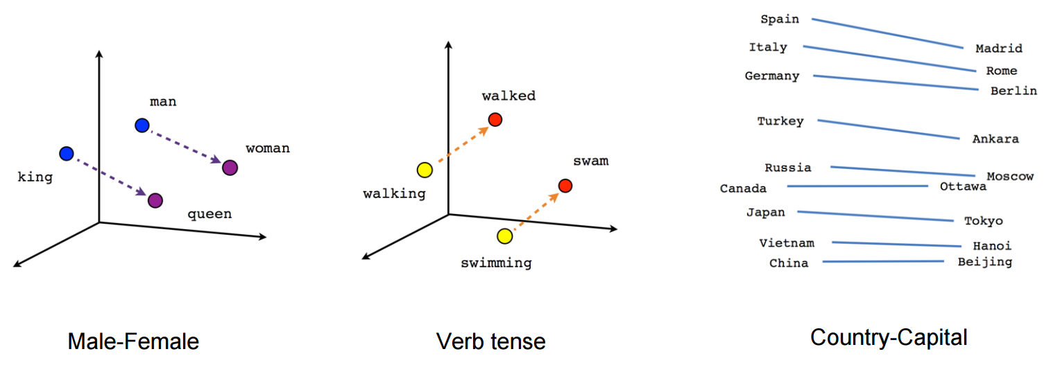
These vectors are a thus lower dimensional, denser representation of our words and they also capture semantic information about words and their relationships to another. Certain directions in the vector space embed certain semantic relationships such as male-female, verb-tense and country-capital relationships between words.

There are algorithms dedicated to learning these embeddings, like Word2vec and Glove, but they can also be just another layer in your neural network.
Build an embedding layer in keras using keras.layers.Embedding.
keras can learn this layer for you, but you can also pretrained embeddings generated by others.
2.2 Recurrent layer
We'd like our neural network to take context into account. When reading the review, it should think what words mean in the relation to the sequence of words seen so far.
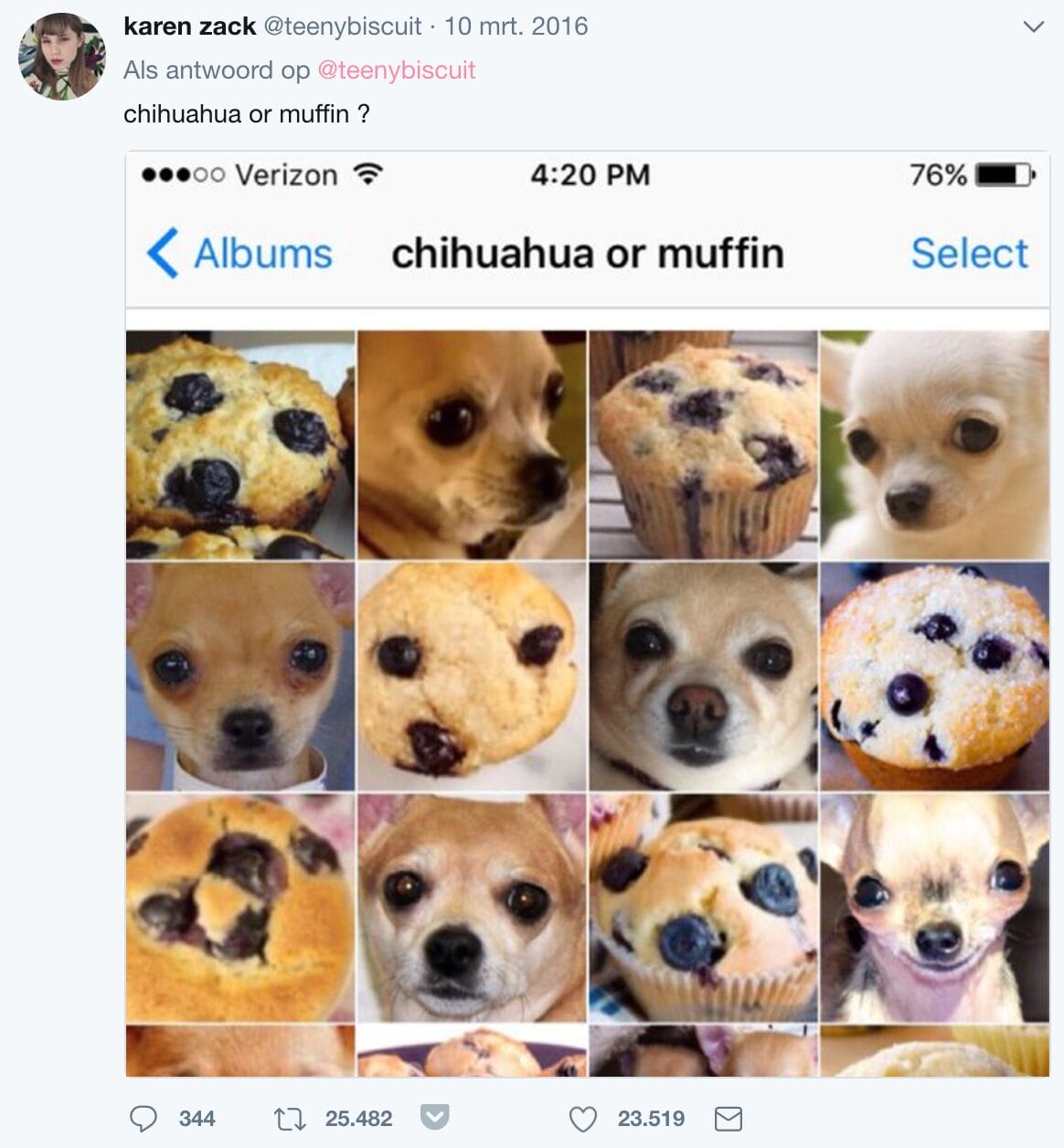
This makes sense for a lot of sequence problems. For instance, if you're looking at a video with a tiny dog house, you're more likely to think that the weird object in the next frame is a chihuahua and not a muffin.

Traditional feedforward networks learn their parameters once and have a fixed state, so they cannot take context in sequences of input data into account. Recurrent neural networks (RNNs) also learn their parameters once, but keep a state depending on the sequence they have seen so far. This makes RNNs well suited for sequence problems, like converting speech to text: translation of a word can be helped by knowing the words that came before.
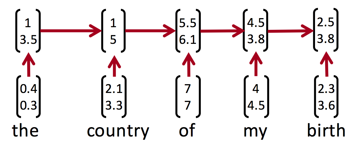
RNNs naturally deal with word order because they go over a sequence of words and keep a memory of the words that have been seen so far. The figure below illustrates how sentiment can change when going through a text. A word can trigger a sentiment that carries on for one or multiple sentences.

If we'd be interested in understanding a document like in the previous example, we could use the following architecture:

The left side of the figure shows a short-hand of the neural network, the right side shows the unrolled version.
In the figure we have:
- (mathbf{x}^{(t-1)}), (mathbf{x}^{(t)}), (mathbf{x}^{(t+1)}): input word vector at time (t).
- (mathbf{h}^{(t-1)}), (mathbf{h}^{(t)}), (mathbf{h}^{(t+1)}): output of the previous time-step (t-1).
At each time-step, the input is the output of the previous time-step (mathbf{h}^{(t-1)}) and a new input word vector (mathbf{x}^{(t)}). Over time we adjust our idea of the document (mathbf{h}^{(t)}) until we've seen all words in the document. This is illustrated in the figure below: we get a new word vector at each time-step and carry over a score.

The final score (mathbf{h}^{(T)}) represents what the neural network has learned about the document after having seen every word. We could, for instance, use the final scores to detect sentiments - and that's exactly what we'll be doing!
We'll use a specific kind of recurrent layer: a LSTM. The Long Short Term Memory neuron are able to learn long-term dependencies and often perform better than standard RNNs. Read this blog if you'd like more info.
keras has multiple types of RNNs, the LSTM layer can be found in keras.layers.LSTM.
2.3 Dense layer
The first layer learns a good representation of words, the second learns to combine words in a single idea, and the final layer turns this idea into a classification.
We will use a simple dense layer from keras.layers.Dense that transforms the idea vectors into a 0 or 1.
The layer will consist of a single neuron that takes all connections and outputs 0 or 1.
3 Training
Time to train our model! The model is a simple sequential model consisting of three layers. The callbacks save the best model and halt training if the model stops improving.
from keras.models import Sequential
from keras.layers import Dense, Embedding, LSTM
from keras import callbacks

# Make our model.
model = Sequential()
model.add(Embedding(NUM_WORDS, 128))
model.add(LSTM(128, dropout=0.2, recurrent_dropout=0.2))
model.add(Dense(1, activation='sigmoid'))

# Callbacks.
checkpoint = callbacks.ModelCheckpoint(filepath='imdb_lstm.h5', verbose=1,
                                       save_best_only=True)
early_stopping = callbacks.EarlyStopping(monitor='val_loss', min_delta=0,
                                         patience=2, verbose=0, mode='auto')

# Compile and train.
model.compile(loss='binary_crossentropy', optimizer='adam',
              metrics=['accuracy'])
model.fit(X_train, y_train, batch_size=64, epochs=20,
          validation_data=(X_test, y_test),
          callbacks=[checkpoint, early_stopping])

score, acc = model.evaluate(X_test, y_test, batch_size=64)

print('Test score:', score)
print('Test accuracy:', acc)

> Test score: 0.44
> Test accuracy: 0.82
The final accuracy is 82% (higher is better) and the binary cross entropy is 0.44 (lower is better).
Is this any good?
What is the baseline score of a more traditional model?
Let's get our good old sklearn out!
from sklearn.feature_extraction.text import TfidfVectorizer
from sklearn.linear_model import LogisticRegression
from sklearn.metrics import accuracy_score, log_loss
from sklearn.pipeline import Pipeline

# Turn the data into strings of integers, because that's how the
# CountVectorizer likes it.
X_train_s = [' '.join(map(str, row)) for row in X_train]
X_test_s = [' '.join(map(str, row)) for row in X_test]

# We'll just use the default values.
pipeline = Pipeline([('counter', TfidfVectorizer()),
                     ('classifier', LogisticRegression())])
pipeline.fit(X_train_s, y_train)

y_sklearn = pipeline.predict(X_test_s)
y_proba_sklearn = pipeline.predict_proba(X_test_s)

print('Test score:', log_loss(y_test, y_proba_sklearn))
print('Test accuracy:', accuracy_score(y_test, y_sklearn))

> Test score: 0.38
> Test accuracy: 0.84
The score and accuracy of our simple model are about the same as those of our neural net!
Neural nets were supposed to be The Futureâ¢, why is it not outperforming our baseline? The dataset is not big enough to learn complex relations. Based on the information the neural net has, it's generalizations can not be better than our simple model. It needs more reviews (and maybe a different architecture) to beat the baseline!
4 Conclusion
This blog post explained some basic NLP concepts and applied them to a simple dataset.
Are you interested in a general and broad introduction to deep learning? Check out our three-day Deep Learning course!
Check out this Stanford course if you'd like to learn how to use Deep Learning for Natural Language Processing.
Written by
Henk Griffioen
Our Ideas
Explore More Blogs
Contact


