
I was curious how unique my new lease car would be in the Netherlands and I wanted to investigate the current trends of new cars. Using the RDW open data portal I have downloaded the dataset of all registered vehicles in the Netherlands. The dataset "Open-Data-RDW-Gekentekende_voertuigen" contains about 16.5M rows and a staggering 96 columns. The total size of the dataset at this moment:
du -h  ~/Downloads/Open_Data_RDW__Gekentekende_voertuigen_*

# 10G  Open_Data_RDW__Gekentekende_voertuigen_20250117.csv
The data has a header and is comma-separated and contains a lot of columns. The last 5 columns are URL references to different datasets. These 5 URLs are repeated for millions of rows. Many low cardinality columns are repeated for all rows, for example, type of car, brand, and 'Taxi indicator' to name a few. A columnar storage format like parquet or DuckDB internal format would be more efficient to store this dataset.

In this blog post we will compare the impact of file formats on this 10Gb CSV dataset. We will compare the following file formats:
- Raw CSV
- Compressed parquet (snappy)
- Compressed parquet (zstd)
- DuckDB internal format
Raw CSV
Let's see what happens when we look for the first and last entry of the dataset using Spark and check the timings.
# Select first column value at the top and bottom of the dataset:

head -n2 ~/Downloads/Open_Data_RDW_* | tail -n1 | cut -d, -f1
tail -n1 ~/Downloads/Open_Data_RDW_* | cut -d, -f1

# Output:
#  first: MR56LN
#  last: MR56LG
Load the dataset in a spark session and create a temporary view to query the dataset.
import os
from pyspark.sql import SparkSession

# Default spark session
spark = SparkSession.builder.appName("CarInspector").getOrCreate()
print(spark.version)  # 4.0.0-preview 2
raw_csv_file = os.path.expanduser(
  "~/Downloads/Open_Data_RDW__Gekentekende_voertuigen_20250117.csv")

# Load dataset as a queryable table
spark.read.csv(raw_csv_file, header=True)
  .createOrReplaceTempView("raw_csv")

first = "MR56LN"
last = "MR56LG"
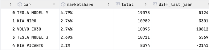
I created an analytical query to view top market share of new cars in the Netherlands:
-- Step 1: group by brand, type and year, count this group

 with cars_brand_per_year as (
    select
        Merk,
        Handelsbenaming,
        substring(cast("Datum eerste toelating" as string), 0,4) as jaar,
        count(*) total
    from raw_csv
    where Voertuigsoort = 'Personenauto'
      and "Datum eerste toelating" >= 20230101
      and "Datum eerste toelating" < 20250101
    group by 1, 2, 3
)

-- Step 2: calculate the market share of the top 30 cars
--   Using a sub-query to calculate the total cars this year.
--   Calculate the diff with the previous year, using a window function.

 select
    jaar, Merk, Handelsbenaming,
    round((total /
           (select count(*) as year_total from raw_csv
            where Voertuigsoort = 'Personenauto'
              and substring(cast("Datum eerste toelating" as string), 0, 4) = 2024)
    ) * 100, 2) || '%' as marketshare,
    total,
    total - lag(total) over (partition by Merk, Handelsbenaming order by jaar) as diff_last_jaar
from cars_brand_per_year
where jaar = 2024 or jaar = 2024 - 1
order by jaar desc, total desc
limit 30
The query including the notebook to load and execute in both Spark and DuckDB can be found on Github as a gist, in case you want to try it yourself.
A small sample of the result, the column car is a concatenation of the brand and type removing the duplicate prefix:
Using the timeit magic command in Jupyter notebook to measure the timings of the queries.
%timeit spark.sql(f"select * from raw_csv where Kenteken='{first}' limit 1").collect()
%timeit spark.sql(f"select * from raw_csv where Kenteken='{last}' limit 1").collect()
%timeit spark.sql(spark_analytical_query).collect()
And compare this with the timing with DuckDB. This is not a fair comparison, because Spark has already inspected the CSV while creating the temporary view. DuckDB will apply the CSV-sniffer to inspect the CSV schema and data types before it can query the data.
import duckdb
print(duckdb.__version__) # 1.1.3

%timeit duckdb.sql(f"select * from '{raw_csv_file}' where Kenteken='{first}' limit 1").fetchall()
%timeit duckdb.sql(f"select * from '{raw_csv_file}' where Kenteken='{last}' limit 1").fetchall()
%timeit duckdb.sql(duckdb_analytical_query).fetchall()
The initial query I have created could not be used in both engines, because the SQL dialect of Spark and DuckDB are not the same. Some differences I have encountered:
- Column references with spaces are different, SparkSQL uses ` (backticks) and DuckDB uses " (double quotes).
substrin only available in SparkSQL,substringin both DuckDB and SparkSQL.- The substring offset in SparkSQL is 0-based, while DuckDB is 1-based. This is annoying.
- Splitting the string in DuckDB is done with
string_split(str, regex)and in SparkSQL withsplit(str, regex), thesplit_part(str, delimit, index)function is equal in both engines. - Selecting the last element of an array is different, SparkSQL uses
element_at(array, -1)and DuckDB usesarray[-1]. - Spark is auto-casting data types more frequent, while DuckDB is stricter in types and requires an explicit cast. See
substring(<bitint>, ...example above.
This is the result of the timings:
| Engine | File format | Timings first row | Timings last row | Timings analytical query |
|---|---|---|---|---|
| Spark | CSV | 31 ms | 9 s | 18 s |
| DuckDB | CSV | 7.5 s | 7.4 s | 8.7 s |
Spark is a lot faster in the first row lookup, but DuckDB is faster in the last row lookup and a lot faster with the analytical query.
Compressed parquet (snappy)
Creating a parquet file from the raw CSV file is straightforward with DuckDB. The default compression algorithm is snappy like in Spark.
duckdb.sql(f"""
    COPY (FROM '{raw_csv_file}')
    TO 'raw_snappy.parquet'
    (FORMAT 'parquet')
""")
The file size of the parquet file is now 1.2G and let's compare the timings of the queries.
| Engine | File format | Timings first row | Timings last row | Timings analytical query |
|---|---|---|---|---|
| Spark | Parquet (snappy) | 140 ms | 700 ms | 1.4 s |
| DuckDB | Parquet (snappy) | 110 ms | 140 ms | 190 ms |
Spark is slower in the last row lookup and significantly slower for the analytical query due to the expensive shuffles. This is required for the distributed nature of Spark. The query plan of the analytical query in Spark is:
== Physical Plan ==
AdaptiveSparkPlan (13)
+- TakeOrderedAndProject (12)
   +- Project (11)
      +- Window (10)
         +- Sort (9)
            +- Exchange (8)                    <-- Shuffle 1x
               +- Project (7)
                  +- HashAggregate (6)
                     +- Exchange (5)           <-- Shuffle 2x
                        +- HashAggregate (4)
                           +- Project (3)
                              +- Filter (2)
                                 +- Scan parquet  (1)
Compressed parquet (zstd)
Let's create a parquet file using the zstd compression algorithm. The ZStandard algorithm is a modern compression algorithm that is optimized for speed and compression ratio developed by Facebook and open-sourced in 2016. It's widely adopted in the industry and supported by many tools and libraries.
duckdb.sql(f"""
    COPY (FROM '{raw_csv_file}')
    TO 'raw_zstd.parquet'
    (FORMAT 'parquet', compression 'zstd')
""")
Which results in:
du -h *.parquet

# 1.2G  raw_snappy.parquet
# 726M  raw_zstd.parquet
I'm amazed that the size is so much smaller (39%) compared to the snappy variant. This size reduction can have positive impact on loading and writing data to disk. And is a cost saver for cloud storage. Let's compare the timings of the queries.
| Engine | File format | Timings first row | Timings last row | Timings analytical query |
|---|---|---|---|---|
| Spark | Parquet (zstd) | 66 ms | 900 ms | 1.3 s |
| DuckDB | Parquet (zstd) | 130 ms | 150 ms | 230 ms |
The Spark first row lookup-query is faster. The analytical query is equal in Spark, but DuckDB is a little bit slower compared to snappy compression in this example.
DuckDB internal format
In the last comparison we will use the DuckDB internal format. This is a binary format that is optimized for query performance. An advantage of the DuckDB internal format is the ability to perform updates and deletes on the data.
# 1: Create a persistent DuckDB database
db = duckdb.connect("duckdb_rdw_cars.db")
# 2: Create an internal table from the CSV file
db.sql(f"""
create table cars as
select *
from read_csv('{raw_csv_file}', header = true)Ã
""")
The DuckDB internal format occupies 1.6G, which is larger than the parquet files. However, the query performance is significantly faster:
| Engine | File format | Timings first row | Timings last row | Timings analytical query |
|---|---|---|---|---|
| DuckDB | Internal | 23 ms | 22 ms | 75 ms |
The analytical query is especially fast in DuckDB compared to the parquet files. Faster than a duck can quack, the query has finished!
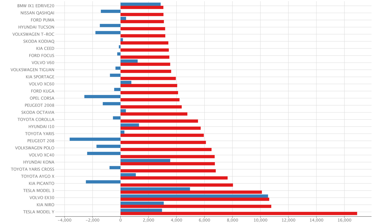
Analytical query
The image is created of the analytical query using PyCharm build-in plotting capabilities:
 RDW dataset: 22-dec-2024
red: absolute number of cars sold in 2024blue: absolute difference with previous year
The results are comparable with autoweek verkoopcijfers, which was slightly out of date at creation time. The date selection for determine the years might also be based on a different column.
Conclusion
In this blog post we have compared the impact of file storage on a 10Gb dataset. Using a "raw" format like CSV is inefficient in storage size and query performance. After compressing the file to parquet using snappy compression the size of the data shrinks significantly (x8,7). The de facto standard for compression is snappy, but zstd is a good alternative with an even better compression ratio (x14,3). Consider using zstd for your parquet files (and delta-lake files) to reduce filesize and thereby cloud storage costs and increase data loading times.
# Change default compression codec from snappy to zstd:
spark.conf.set("spark.sql.parquet.compression.codec", "zstd")
DuckDB is a good alternative for Spark when working on analytical queries on reasonable datasize. Best performance is achieved with the DuckDB internal format.
In case you are wondering about my new lease car. It's at position 137, the Mazda 3 with a market share of the 0.148% in 2024. Which is a relative unique car.
You can view the notebook-gist on Github.
Written by

Alexander Bij
Our Ideas
Explore More Blogs


Contact