The challenges of molecular property datasets

One of the most crucial steps in building machine learning models to predict molecular properties is splitting our data into training, validation, and test sets. A well-thought-out splitting strategy ensures that our model generalizes well to unseen data and provides reliable performance metrics. Often, we are not just interested in a single property but in predicting multiple properties simultaneously. Not all properties are created equal, some are more abundant in our datasets than others. If not handled properly, this imbalance can lead to biased models.

In this blog post, we will explain why there is an imbalance in molecular property datasets and explore strategies for validating data splits. In summary there are two main factors to control for when splitting data for molecular properties: data distribution and data availability. We show how to test if the data distribution is similar between the different sets using the Kolmogorov-Smirnov test. We also show how to test if the data availability is similar using the proportions z-test. This ensures that our test (and validation) set is representative of the training set, leading to more reliable model evaluation.

Understanding the Data

We will be working with data from the Open Polymer Challenge. It consists of various molecular structures represented as SMILES strings, along with multiple target properties that we aim to predict. These include: - glass transition temperature (Tg) - fractional free volume (FFV) - thermal conductivity (Tc) - polymer density (De) - radius of gyration (Rg)

kaggle competitions download -c neurips-open-polymer-prediction-2025

When we look at the distribution of these properties, we notice that some properties are more frequently represented in the dataset than others.

from pathlib import Path
import pandas as pd


csv_path = Path("./neurips-open-polymer-prediction-2025/train.csv")
train_df = pd.read_csv(csv_path)
train_df.drop(columns=["id", "SMILES"]).describe()

Understanding Data Availability Patterns

There are two ways of collecting molecular property data: through physics simulations (also known as Molecular Dynamics (MD) simulations) and experimental measurements. There are several challenges in collecting polymer property data depending on the method used. The availability of polymer property data varies significantly between physics simulations and experimental measurements, with each property presenting unique challenges in data generation. Since the open polymer challenge dataset contains simulated or computational data, we will focus here on understanding the implications of the computational challenges and its impact on the availability of data for different properties. In the appendix, we provide an overview of the challenges of experimental data generation.

Physics Simulation Data Generation

For physics simulations, data generation feasibility follows: radius of gyration ≈ density > fractional free volume > glass transition temperature > thermal conductivity, based on computational requirements and methodological complexity.

Glass Transition Temperature (Tg) - Moderate Complexity

Physics simulations can reliably generate glass transition temperature data through molecular dynamics (MD) methods, though with some important limitations. Glass transition temperature determination in MD simulations involves cooling rate dependencies and systematic temperature offsets [1, 2].

The computational protocol involves density versus temperature analysis during cooling simulations, where Tg is identified from the intersection of two linear fits in the density-temperature curve [1, 3]. Despite the systematic offset, MD simulations can successfully capture relative trends and provide consistent rankings of polymer Tg values [3, 4].

Fractional Free Volume (FFV) - High Computational Feasibility

FFV is one of the most accessible properties for computational generation, with extensive high-throughput molecular dynamics datasets already available [5, 6, 7]. Computational FFV determination uses geometric analysis methods such as Delaunay tessellation or probe particle insertion to quantify void space in polymer structures [5, 7, 8].

Recent studies have generated FFV data for thousands of polymers through automated MD simulation protocols. Ma et al. created datasets with over 6,500 homopolymers and 1,400 polyamides [5], while Wang et al. developed datasets with 1,683 polymers that were then applied to screen over 1 million hypothetical structures [6]. The computational method provides excellent scalability for high-throughput screening applications.

Thermal Conductivity (Tc) - Computationally Intensive but Feasible

Thermal conductivity calculations through MD simulations are computationally demanding but well-established [9, 10, 11, 12]. The property requires equilibrium molecular dynamics simulations with careful attention to system size effects and long simulation times to achieve statistical convergence [10, 12].

High-throughput studies have successfully generated thermal conductivity data for hundreds of polymers [10, 11, 12]. Ma et al. calculated thermal conductivity for 365 polymers using MD simulations, then used this data to train machine learning models for screening larger databases [10]. The computational cost is higher than FFV calculations but remains feasible for building substantial datasets.

Polymer Density (De) - Straightforward Calculation

Density is computationally straightforward to obtain from MD simulations [13, 14]. It requires standard NPT (constant pressure and temperature) ensemble simulations where density is calculated from the mass and volume of the simulation cell [13]. The RadonPy automated framework demonstrates successful high-throughput density calculations for over 1,000 unique polymers [13].

Density calculations show good agreement with experimental values when proper equilibration protocols are followed [13]. The main challenge involves achieving proper equilibration, particularly for complex polymer systems that may require extended annealing procedures [14].

Radius of Gyration (Rg) - Easily Computed

Radius of gyration is among the most accessible properties in MD simulations [13, 15, 16]. It's calculated directly from atomic coordinates using a simple mathematical formula that measures the distribution of mass around the center of mass [13, 16]. The calculation requires minimal computational overhead and can be obtained from any equilibrated polymer structure.

Rg serves as an important equilibration criterion in polymer simulations, with typical convergence requirements of less than 1% relative standard deviation [13]. This property is routinely calculated in polymer simulation studies and presents no significant computational barriers.

Factors to Control For

So, in addition to the standard practice of controlling for the distribution of the target property, we also need to take into account the availability of the different properties.

Testing for Distribution

We test if there is a difference between the train and test distribution using the Kolmogorov-Smirnov test.

from scipy.stats import ks_2samp


def ks_test_feature(set_a, set_b):
    stat, p_value = ks_2samp(set_a.dropna(), set_b.dropna())
    return stat, p_value

Testing for Data Availability

To test the difference in the proportion of missing values between two sets, we can use the proportions z-test.

from statsmodels.stats.proportion import proportions_ztest


def run_proportions_ztest(set_a, set_b):
    counts = np.array([set_a.notnull().sum(), set_b.notnull().sum()])
    nobs = np.array([set_a.size, set_b.size])
    stat, pval = proportions_ztest(counts, nobs)
    return stat, pval

Splitting the Data

We load in the training data of the Open Polymer Challenge and split it into a training (80%), validation (10%), and test set (10%). Since there is limited data available for some properties and we need enough training examples to learn from and limit the need of retraining on the whole dataset, we use a 80-10-10 split. When using less data hungry methods 60-20-20 may be an option. Since we are testing for similarity of data distribution and availability, we ensure that the splits are representative and can get away with fewer samples in the validation and test sets.

import pandas as pd
from sklearn.model_selection import train_test_split


# 1. split off 10% for dev_test
temp_df, dev_test = train_test_split(
    train_df,
    test_size=0.1,
    random_state=SEED,
    shuffle=True
)

# 2. split the remaining 90% into 80% train and 10% valid
dev_train, dev_val = train_test_split(
    temp_df,
    test_size=0.111,  # 0.111 * 0.9 = 0.1 of the original
    random_state=SEED,
    shuffle=True
)

Note that we use random sampling here since we want to ensure that the test sets is representative of the overall data distribution. An alternative strategy for splitting molecular data is scaffold splitting, which ensures that the chemical scaffolds in the test set are not present in the training set. The idea is to test the model's ability to generalize to completely new chemical structures. While there are python packages that make it look easy, greglandrum and practicalcheminformatics motivate why scaffold splitting is not as straightforward as it seems. A subtle difference between our validation method and scaffold splitting is that we focus on the distribution of the properties and their availability, rather than the chemical structure of the molecules.

Test if the Distribution is Similar

We first try SEED=42 and check if the distribution of the different properties is similar between the train and test set:

for feature in dev_train.drop(columns=["id", "SMILES"]).columns:
    stat, p_value = ks_test_feature(dev_train[feature], dev_test[feature])
    print(f"K-S Test for {feature}: Statistic={stat:.4f}, p-value={p_value:.4f}")

SEED=42
K-S Test for Tg: Statistic=0.1779, p-value=0.1948
K-S Test for FFV: Statistic=0.0212, p-value=0.9299
K-S Test for Tc: Statistic=0.0893, p-value=0.7483
K-S Test for Density: Statistic=0.0833, p-value=0.8756
K-S Test for Rg: Statistic=0.1543, p-value=0.1895

All p-values are above 0.05, indicating that we fail to reject the null hypothesis that the two samples come from the same distribution. In other words, the distributions of the properties in the dev_train and dev_test sets are similar enough.

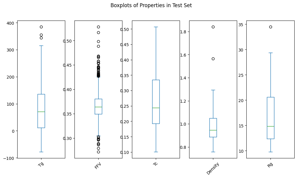
Which we can confirm by visual inspection of the distributions: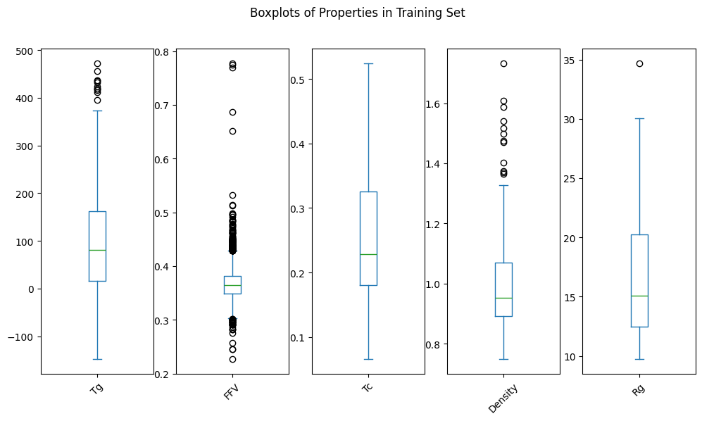

Test if the Data Availability is Similar

Next we check if the data availability is similar between the train and test set:

for feature in dev_train.drop(columns=["id", "SMILES"]).columns:
    stat, pval = run_proportions_ztest(dev_train[feature], dev_test[feature])
    print(f"Proportions Z-Test for {feature}: Statistic={stat:.4f}, p-value={pval:.4f}")

SEED=42
Proportions Z-Test for Tg: Statistic=1.9714, p-value=0.0487
Proportions Z-Test for FFV: Statistic=-2.2804, p-value=0.0226
Proportions Z-Test for Tc: Statistic=1.9360, p-value=0.0529
Proportions Z-Test for Density: Statistic=1.4778, p-value=0.1395
Proportions Z-Test for Rg: Statistic=1.3515, p-value=0.1765

Here, we see that the p-values for Tg and FFV are below 0.05, indicating that we reject the null hypothesis that the proportions of missing values are the same in both sets. In other words, the availability of Tg and FFV data is significantly different between the train and test sets.

Which we can confirm if we look at the missing value proportions:

We try again with SEED=0:

SEED=0
Proportions Z-Test for Tg: Statistic=0.1784, p-value=0.8584
Proportions Z-Test for FFV: Statistic=-1.3942, p-value=0.1633
Proportions Z-Test for Tc: Statistic=0.0657, p-value=0.9476
Proportions Z-Test for Density: Statistic=-1.3214, p-value=0.1864
Proportions Z-Test for Rg: Statistic=-1.3214, p-value=0.1864

This time, all p-values are above 0.05, indicating that the proportions of missing values are similar in both sets.

Conclusion

When splitting data for molecular properties, especially when dealing with multiple properties with varying levels of representation, it's crucial to ensure that both the distribution of the properties and the missing value patterns are similar across the training, validation, and test sets. We showed how to use the Kolmogorov-Smirnov test to compare distributions and the proportions z-test to compare availability.

We have explained the observed patterns in polymer property datasets, where certain properties have substantially more missing values than others. The computational advantages for FFV and Rg, combined with experimental limitations for these properties, create datasets heavily skewed toward simulation-derived data for these properties.

The next step is training your model and evaluating its performance on the validation and test sets. While the topic of training ML models for molecular property prediction is beyond the scope of this blog post, we encourage you to think about the metric used to evaluate these models. Given the learnings from this post, a weighted metric that accounts for the varying availability of properties may be more appropriate than a simple average.

Appendix

Which sets to compare?

Note that the difference between the train and the test distribution is compared, and not one of the subsets is compared against the whole dataset. The test statistic assumes independent samples. If one set were a subset of the other, this assumption would be violated.

Completeness

For sake of completeness, we also calculated the Kolmogorov-Smirnov test statistic and p-value when SEED=0:

SEED=0
K-S Test for Tg: Statistic=0.0808, p-value=0.9137
K-S Test for FFV: Statistic=0.0220, p-value=0.9102
K-S Test for Tc: Statistic=0.1284, p-value=0.2133
K-S Test for Density: Statistic=0.1112, p-value=0.3953
K-S Test for Rg: Statistic=0.1612, p-value=0.0708

Again, all p-values are above 0.05, indicating that we fail to reject the null hypothesis that the two samples come from the same distribution.

Experimental Data Generation Challenges

It is worth understanding the experimental challenges as well, since they are different from the computational ones and there are experimental datasets available as well. Experimental methods face increasing challenges in the order: density < thermal conductivity < glass transition temperature < fractional free volume < radius of gyration. Therefore, properties like density and thermal conductivity may show better experimental representation despite computational accessibility.

Glass Transition Temperature (Tg) - Significant Experimental Challenges

Experimental Tg determination faces substantial difficulties, particularly for rigid conjugated polymers [17, 18, 19]. Traditional differential scanning calorimetry (DSC) methods often fail to detect clear glass transitions in donor-acceptor conjugated polymers due to extremely small changes in specific heat capacity (Δcp) [17, 19]. Values can drop from 0.28 J·g⁻¹K⁻¹ for flexible polymers like polystyrene to 10⁻³ J·g⁻¹K⁻¹ for rigid conjugated polymers [17].

The challenges stem from rigid backbone structures and semicrystalline nature of many polymers, which reduce the magnitude of thermal signatures [17, 19]. Experimental protocols require specialized techniques including physical aging experiments, cooling rate dependency studies, and complementary dynamic mechanical analysis to confirm Tg values [18, 19].

Computational vs Experimental

Simulated Tg values typically overestimate experimental measurements by 80-120 K due to the much faster cooling rates in simulations (10⁹ K/s) compared to experiments (10⁻²-10⁻¹ K/s) [1]. Take this into account when combining simulated and experimental Tg data.

Fractional Free Volume (FFV) - Indirect Experimental Methods

Experimental FFV determination relies on indirect methods with significant limitations [7, 8]. Positron annihilation lifetime spectroscopy (PALS) provides relative measurements but requires calibration and involves assumptions about void shape [8]. Group contribution methods using van der Waals volumes introduce ambiguities in parameter selection and structural group definitions [7].

Recent advances have updated Bondi's group contribution method, but experimental validation remains challenging due to the need for direct free volume measurement techniques [7]. The semi-empirical nature of experimental approaches creates uncertainties in absolute FFV values.

Thermal Conductivity (Tc) - Measurement Complexity

Thermal conductivity measurement in polymers presents significant experimental challenges [20, 21, 22]. The property is "notoriously difficult to measure" for polymeric liquids and solids[22]. Key challenges include eliminating convection effects, ensuring proper thermal contact, and managing temperature gradients [20, 21].

Measurement uncertainties can reach ±20.7% for semi-crystalline polymers under atmospheric pressure conditions [20]. The complexity increases with processing conditions relevant to industrial applications, requiring specialized high-pressure, high-temperature equipment [20]. Sample preparation and thermal history effects add additional variability [21].

Polymer Density (De) - Precision and Sample Challenges

Experimental density measurement faces precision challenges, especially for small or heterogeneous samples [23, 24]. The Archimedes method shows limitations for thin-wall specimens, while precision density measurements require careful control of temperature, humidity, and sample preparation [23, 24].

Variations within samples and the need for representative sampling create additional complications [23]. For polymer systems under processing conditions, specialized pressure-volume-temperature (pvT) equipment is required, adding complexity and cost [20].

Radius of Gyration (Rg) - Limited Direct Experimental Access

Radius of gyration lacks direct experimental measurement techniques for bulk polymer systems. While light scattering can provide Rg information for polymers in solution, this represents a different state than bulk polymer properties relevant to most applications [16]. Small-angle neutron scattering and X-ray scattering can provide structural information but require specialized facilities and complex data interpretation.

The property is primarily accessible through computational methods, creating a significant data gap for experimental validation of simulation predictions.

References

Banner image credits: Lone Thomasky & Bits&Bäume / Distorted Lava Flow / Licenced by CC-BY 4.0

The code can be found on our GitHub.