In this post, we’ll cover tracking changes, as well as comparing and tracking the deployment of Machine Learning models using MLflow library. We’ll later set up resources in the Azure Cloud so we can provision our model, as well as create the Azure DevOps pipeline to deploy a new model by just pushing it to the Azure GIT repository. This will highlight just how easy it is to get set-up with ML – it’s not as long or as difficult as you think, if you know what you’re doing!
We won’t focus on hypertuning the model parameters, feature exploration or cleaning the data. In our example, we’ll use the “Richter’s Predictor: Modeling Earthquake Damage” challenge hosted by DrivenData.
IT Application Development Process
When we develop a desktop application, mobile product or website, we always start by planning the features that we’re are going to deliver (it’s part of essential product design). We then program and deploy them to the server in a continuous manner.
By “continuous” I mean that, from all the features that are planned to be delivered, we select a small subset and work on it. After work is done and tested, the changes are deployed to the server, by either developers or deployment team. This is known as Continuous Integration, Continuous Delivery (CI/CD) and is part of the DevOps approach.
Because we work this way, the client can start using the features we already completed, while we work on another subset of features. To keep track of all the changes in the codebase, we always want to use some sort of version control system, like Git, for example. Why? someone might ask. In complex applications, even the smallest changes in code that’s already written – and required to progress working on the current feature – can accidentally break some other feature. Similarly, if there was some requirement change followed by adjustments in the codebase, the other part of the application may have been strictly dependent on how it worked before the modification. That part of the now broken code, obviously, will not work after the change, but that can sometimes slip away during tests.
These situations happen sometimes, and that’s why we want to be able to see all the changes, to be able to see all previous work that has been done and find the culprit that caused the feature break. This also allows us to easily rollback to previous versions, if required. After all the features are delivered, there is not much more to do, so we switch to maintenance and only fix bugs without developing new features.
Is Machine Learning Model Development That Different?
While the application implementation is in the iterative stage, we can plan exactly what needs to be done. The model implementation, on the other hand, is a more exploratory process and, as such, we don’t really know what will need to be done in order to achieve the best results.
Of course, we can plan some of the main steps, such as integrating data, data analysis, data validation, training or building the model and even deployment. But we can rarely exactly tell what needs to be done, as there is always a place to improve the model even further.
After we build one model, we try to build the next one to achieve even better results. We can use different learning techniques, change the hyperparameters of the current algorithm a little (so it better reflects reality), try integrating new data, or maybe try a radically different approach. There are endless possibilities to try and determine if they help with our model accuracy.
However, just like in application development, we want to keep track of the work that was already done, so we don’t do the same things twice – or more! We also need to be able to compare the results, because combining different solutions can often lead to an even better one. Yet keeping all the code for different models, as well as all parameters and results in multiple directories and excel spreadsheets, would be real pain.
It’s also rare to work in one-person teams, so we also need to be able to reproduce our experiments or share them with other data scientists. Deployment of the new model is another thing we need to handle.Manually creating docker images and deploying to the server are not that difficult, but it takes precious time we could spend testing another model. So we would like some easy, effortless and automatic deployment process.
MLflow to rescue
MLflow focuses on three basic goals:
- tracking the experiments, aka parameters
- results
- other artifacts
Packaged ML code, in a reusable and reproducible form, allows for sharing with other data scientists and moving the model to production, as well as helping with deployments, as it supports a variety of libraries and Cloud platforms. However, in this article, the main focus will be on tracking the model and Cloud deployment.
Fortunately, that covers the previously mentioned problems mentioned regarding tracking, sharing, and deployment. MLflow is fairly simple to use and doesn’t require so many changes in code, which is a big plus. It also allows for storing the artifacts of each experiment, such as parameters and code, as well as models stored both locally and on remote servers/machines. If that wasn’t enough, there’s a very nice interface for comparing the experiments that have built-in charts, so you don’t have to produce them yourself.
Finally, it also supports many models from libraries such as scikit-learn, Keras, PyTorch or ONNX, alongside languages such as Python, R, Java and REST API, as well as the command line.
Let’s Get Started
We’ll use this simple example to show how to track a model and deploy it to the Azure Cloud using Python. In the below code, we train a very simple sequential model using Keras library. During the neural network learning process, data is presented to the neural network algorithm multiple times. One forward and one backward pass of all training examples to the model is called an epoch. After each single run of the neural network, we’ll log each epoch’s accuracy and loss on both training and test data sets, parameters that were used and save the neural network model.
To run the script, we’ll need to install a few libraries, so let’s install these first:
Now that we have the required libraries, let’s look at the script.
Let’s skip the boring loading data step and jump immediately to the ‘run_learning ’ method.
First, we save all the parameters that were passed to the method that we’ll be exploring shortly. Next, we set run_learningthe main directory, so all the artifacts are saved in the base directory, not where jupyter notebook is running, after that, we set the experiment name and start it up. If we want to set the directory locally, we need to add the prefix ‘file:’ before the path, for HTTP URI (Uniform Resource Identifier), we add ‘https:’ and, if we want to use a databricks workspace, we add ‘databricks://’. Instead of a ‘with … as …’ clause, we can assign it to the variable, but we need to remember to close the experiment manually, using the ‘end_run’ method then. The ‘with … as …’ notation is error-prone, hence we’ll stick to this approach.
The first thing we do after starting the experiment is logging parameters using the ‘mlflow.log_param‘ method but, of course, the logging order is not important – as long as it stays in the experiment scope. After that, we create a temporary directory for artifacts, alongside creating, fitting, training and scoring the Keras model.
Once this is done, we log all the results with ‘log_metric’ in a similar manner as described already. MLflow doesn’t support arrays out of the box, so we need to use the three-parameter method. We enumerate the array and log each epoch separately in the loop.
Last of all, we save the model and instruct the MLflow to move the artifact to the earlier specified path, and end with the process by removing the temporary files.
Now that we have explained the script, let’s run it in a jupyter notebook and see the MLflow UI.
Here’s an example result after running the learning script a few times with different parameters.
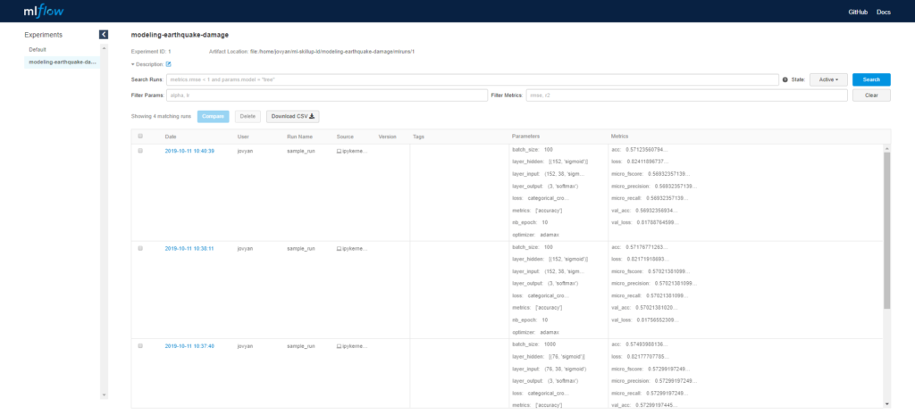
We can split each parameter/metric into separate columns by clicking on the parameter name
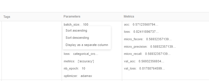
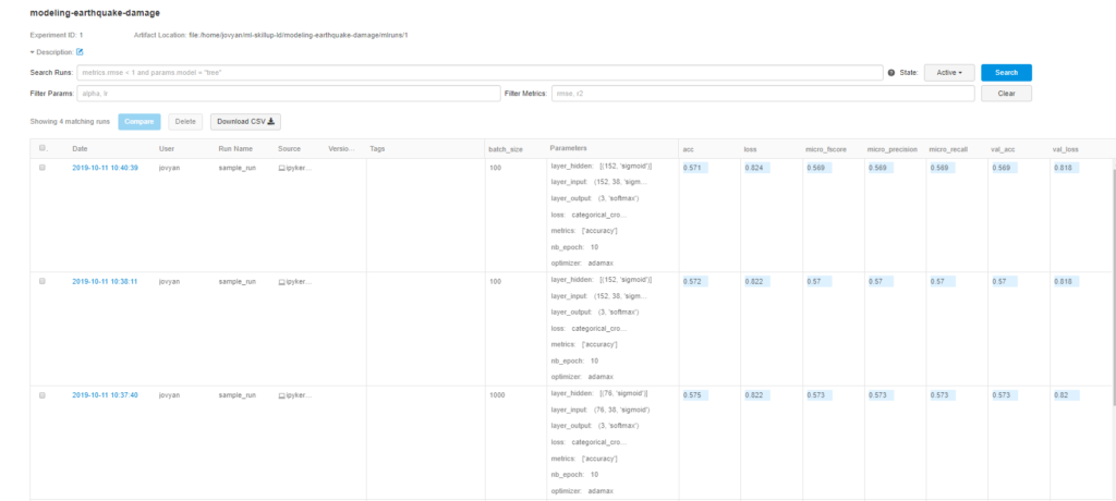
For example, like so:
We can take a look at one experiment by clicking on the date hyperlink, where we can see all logged parameters, metrics and artifacts. The artifact can also be downloaded after being selected.
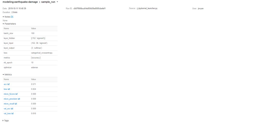

We can also peek at the loss metric that was logged in the loop by clicking on it.

Another great thing is the out-of-the-box comparison between different run results. To do this, we just need to check the checkboxes and click the ‘compare’ button.
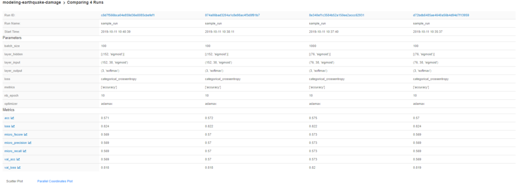

We can also compare the accuracy changes in each epoch between the selected models.

After we compare all the results and select the best model, we can download the archived version we saved as an artifact, which will be used later on.
Deploying The Keras Model
We decided to host our model in the Azure Cloud, so we need to configure our Azure services to be able to host the model we created in the last step. Let’s jump into this right now!
First, head to the Azure portal and log in. If you don’t have an account, you can create it a few simple steps. Now, let’s create a new resource group. This will be used to group all resources, such as our application, image container and so one. Click on the ‘Resource groups’ and later click ‘Add’, give the resource group a name, select the region and click ‘Review + create’ followed by ‘Create’.
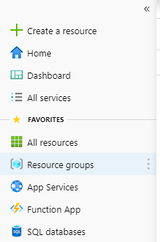
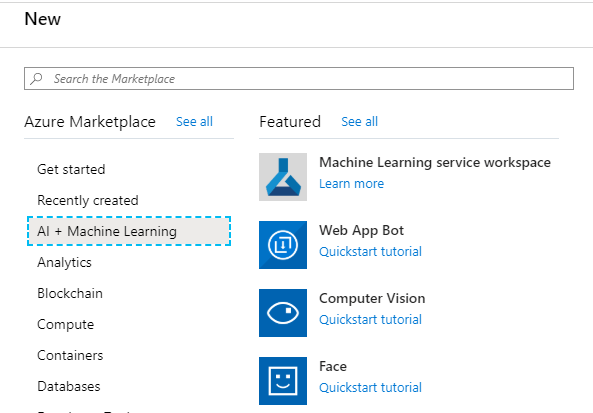
Now click the ‘Create resource’ on the left panel, then ‘AI + Machine Learning’ and ‘Machine Learning service workspace’. Give your namespace a name, select a previously created resource group and create it. Then, just wait untill Azure completes the creation of these resources.
Now let’s add the Service principal that will allow us to access our resources from our code. First of all, click on ‘Azure Active Directory’ in the left panel, then on ‘App registrations’, before clicking the ‘Add’ button and creating the application.
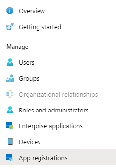
We’ll be redirected to the details of the app registration we just created. Copy the Application (client) ID and Directory (tenant) ID, as it’ll be needed later. Now, click on the ‘Certificates & secrets’ and create a secret by clicking the ‘New client secret’. Copy the secret somewhere, as it’ll also be needed later on.
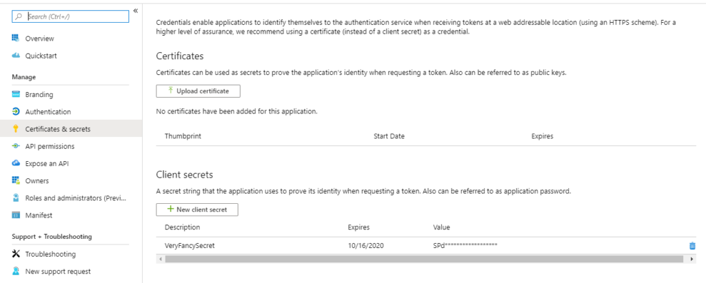
Now we have the service principal that we can use to log in from the code, we need to give it access to all the resources created earlier. Let’s head back to Resource groups and select the resource we created earlier, followed by ‘Access control (IAM)’.

We can check who can access our resources by viewing role assignments, so let’s click ‘view’. Now, we should see all applications, users and groups that have access to this resource group. Access to all resources in this resource group is inherited, so to access earlier created Machine learning services, we just need to add our service principal here.
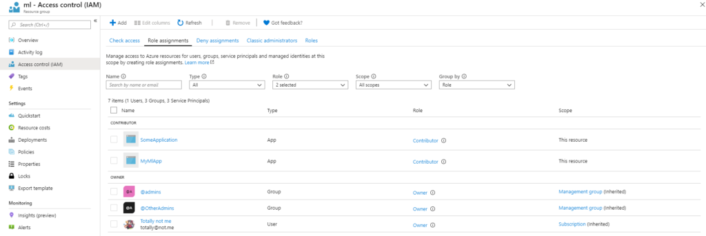
Let’s go ahead and click on the ‘Add’ button, followed by ‘Add role assignment’. A new panel should appear where we select the role to determine/indicate who will get that role. It’s recommended to set the role as a contributor, so it can manage everything, but restrict changing access rights to the resource. Then, we want to select the app we created and click save. Now we set up everything, including a few more configuration settings that need to be set:
- location – this is just the location for our resources, so let’s make sure it’s the same as the group location
- resource_group – the name of the resource group that was created
- workspace_name – the name of the workspace created
- subscription_id – subscription id (just search subscription in the top bar)
- account_name – the name of the storage account that was created in the resource group (go to resource groups -> select resource -> and look for storage account and copy its name)
- account_key – Access key to the storage account (found under the Access Keys tab in the storage account)
- service_principal_id, service_principal_password, and tenant_id can be accessed through App registrations in Azure’s Active Directory.
- tenant_id is the “Directory (tenant) ID”
- service_principal_id is “Application (client) ID”
- service_principal_password is the “client secret” we created in the “Certificates & secrets” tab
Now, let’s take a look at the deployment script.
In the beginning, we import secure variables, such as account name, principal id, and password, from the environment. Next, we unpack the model, followed by the loading model, to check if it is valid. Later, we create an authentication object using the service principal (the application we created earlier) id and password.
After this, we create or get a workspace, with the ‘exist_ok’ property set to True, which allows us to continue without creating a workspace if it already exists; otherwise, we’ll get an exception. In the next step, the image is being built, followed by its deployment.
Before running the script, insert a path to your model!
Now we know how to deploy the model, so let’s make it happen automagically!
Azure DevOps Pipeline Set-Up
We want to set-up a pipeline that will deploy our model to the Azure Cloud after it’s being pushed to the repository.
Let’s head to the Azure DevOps page and log in. First, we need to create a project if we haven’t already. After that, let’s import the repository. Go to Repos, click Import and paste the template repository URL.
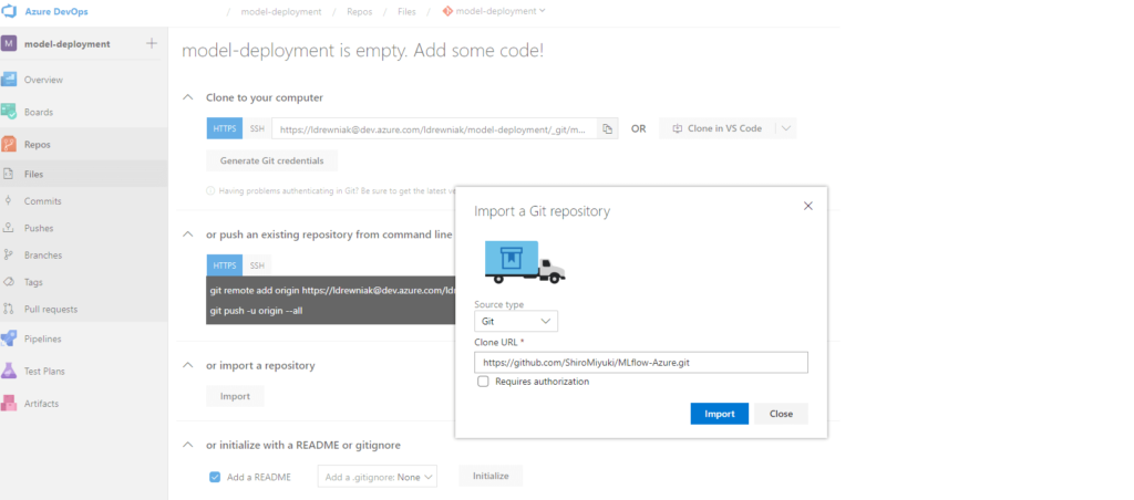
Now, let’s create the pipeline. Go to Pipelines, New pipeline, Azure Repos Git and select repository. You should see the YAML code now and, in right top corner, click variables and add the variables that were listed earlier – remember to check the sensitive ones as a secret!
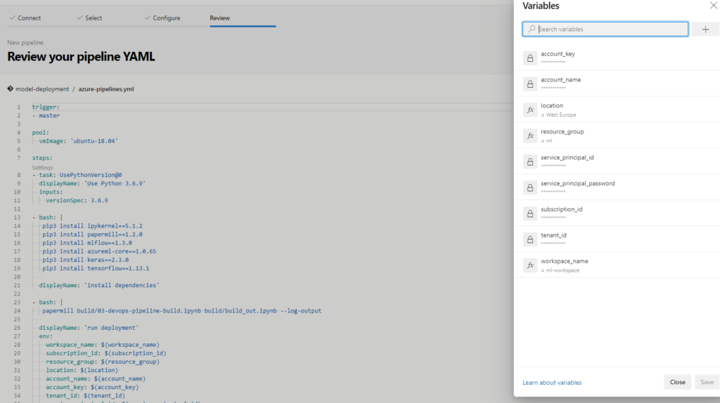
Save the variables and click ‘Run’. Now, while the deployment is running, let’s peek at YAML.
The pipeline has just a few steps. First, it selects the virtual machine version, then it selects the Python version and installs all the required dependencies, followed by running the deployment notebook, complete with all variables added to the environment. Finally, in the end, it prints out the scoring URL.
As for the deployment script, this is very similar to the script we covered earlier, as there are only a few changes. After importing the secrets, we scan the directory and select the model with the highest version. The model names should be as follows v.zip.
In the last step of the pipeline, we can see the URL where the model is provisioned.

Summary
So, what have we learned? We’ve shown how to track ML model changes and compare the models between each others, using the MLflow library. We also learned how to set up Azure resources, so we can deploy the model from code. After that, we covered setting up the Azure DevOps pipeline.
Now, if we want to deploy a new model, we just need to push it to our GIT repository and it’ll build an image, save to a container registry and deploy it to the Azure Cloud.
I hope this shows just how easy it is to set up a range of ML applications and solutions. Paired with the Cloud – not just Azure, but also AWS and Google Cloud Platform, it’s very possible to get versatile and exceptional ML applications for any business.
Business Perspective
Thanks to Cloud platforms like Azure, we now have easy access to test and track our Machine Learning models. In addition to cost-effective resource management, this enables businesses to easily get started with ML and start gaining the benefits as quickly as possible.


