Introduction
LLM’s can be supercharged using a technique called RAG, allowing us to overcome dealbreaker problems like hallucinations or no access to internal data. RAG is gaining more industry momentum and is becoming rapidly more mature both in the open-source world and at major Cloud vendors. But what can we expect from RAG? What is the current state of the tech in the industry? What use cases work well and which are more challenging? Let’s find out together!
Why RAG
Retrieval Augmented Generation (RAG) is a popular technique to combine retrieval methods like vector search together with Large Language Models (LLM’s). This gives us several advantages like retrieving extra information based on a user search query: allowing us to quote and cite LLM-generated answers. In short, RAG is valuable because:
- Access to up-to-date knowledge
- Access to internal company data
- More factual answers
That all sounds great. But how does RAG work? Let’s introduce the Levels of RAG to help us understand RAG in increasing grades of complexity.
The Levels of RAG
RAG has many different facets. To help more easily understand RAG, let’s break it down into four levels:
 Level 1 Level 1Basic RAG |  Level 2 Level 2Hybrid Search |  Level 3 Level 3Advanced data formats |  Level 4 Level 4Multimodal |
|---|
Each level adds new complexity. Besides explaining the techniques, we will also look into justifying the introduced complexities. That is important, because you want to have good reasons to do so: we want to make everything as simple as possible, but no simpler [1].
We will start with building a RAG from the beginning and understand which components are required to do so. So let’s jump right into Level 1: Basic RAG.
Level 1: Basic RAG

Let’s build a RAG. To do RAG, we need two main components: document retrieval and answer generation.
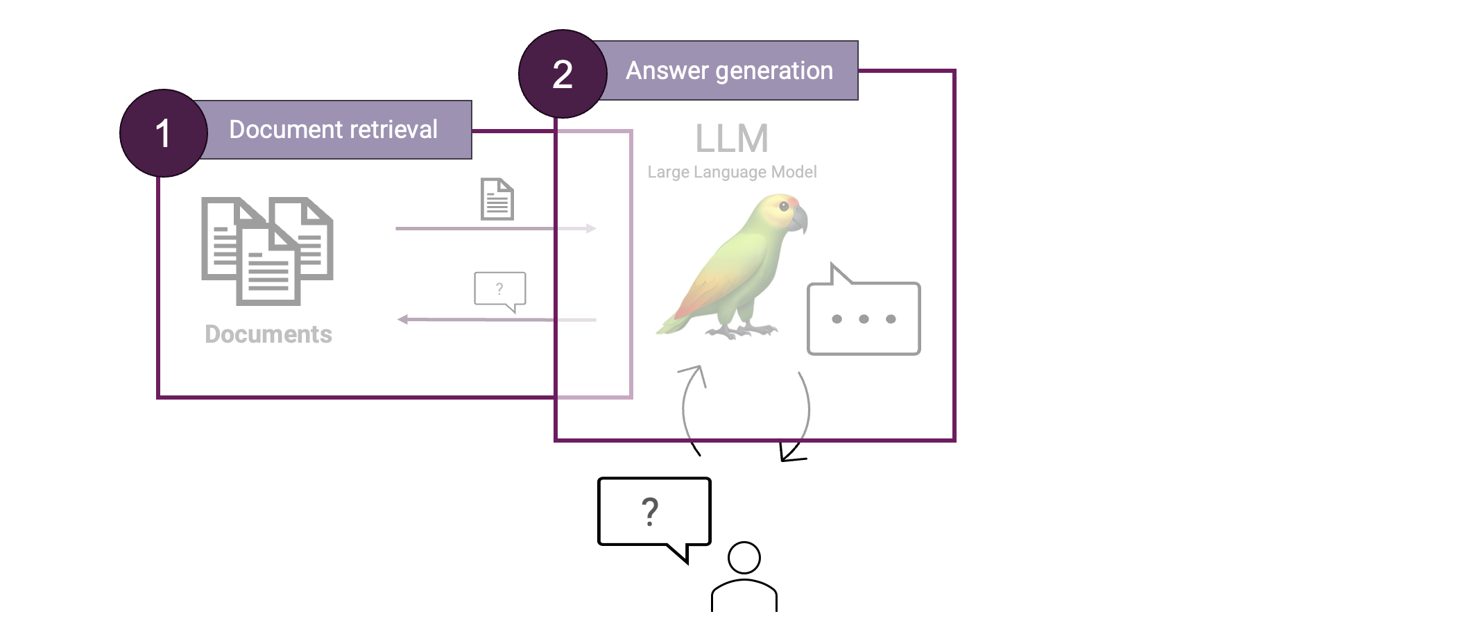
In contrast with a normal LLM interaction, we are now first retrieving relevant context to only then answer the question using that context. That allows us to ground our answer in the retrieved context, making the answer more factually reliable.
Let’s look at both components in more detail, starting with the Document retrieval step. One of the main techniques powering our retrieval step is Vector Search.
Vector Search
To retrieve documents relevant to our user query, we will use Vector Search. This technique is based on vector embeddings. What are those? Imagine we embed words. Then words that are semantically similar should be closer together in the embedding space. We can do the same for sentences, paragraphs, or even whole documents. Such an embedding is typically represented by vectors of 768-, 1024-, or even 3072 dimensions. Though we as humans cannot visualize such high-dimensional spaces: we can only see 3 dimensions! For example sake let us compress such an embedding space into 2 dimensions so we visualize it:

Note this is a drastically oversimplified explanation of vector embeddings. Creating vector embeddings of text: from words up to entire documents, is quite a study on its own. Most important to note though is that with embeddings we capture the meaning of the embedded text!
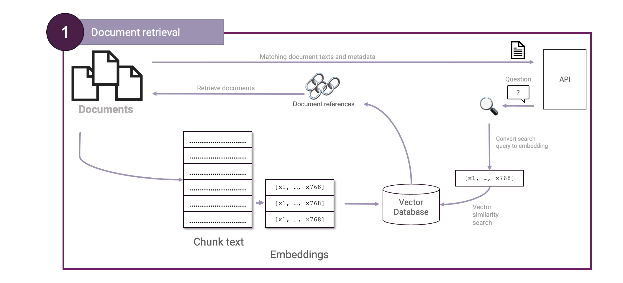
So how to use this for RAG? Well, instead of embedding words we can embed our source documents instead. We can then also embed the user question and then perform a vector similarity search on those:

Great! We now have the ingredients necessary to construct our first Document retrieval setup:

Next is the Answer generation step. This will entail passing the found pieces of context to an LLM to form a final answer out of it. We will keep that simple so will use a single prompt for that:
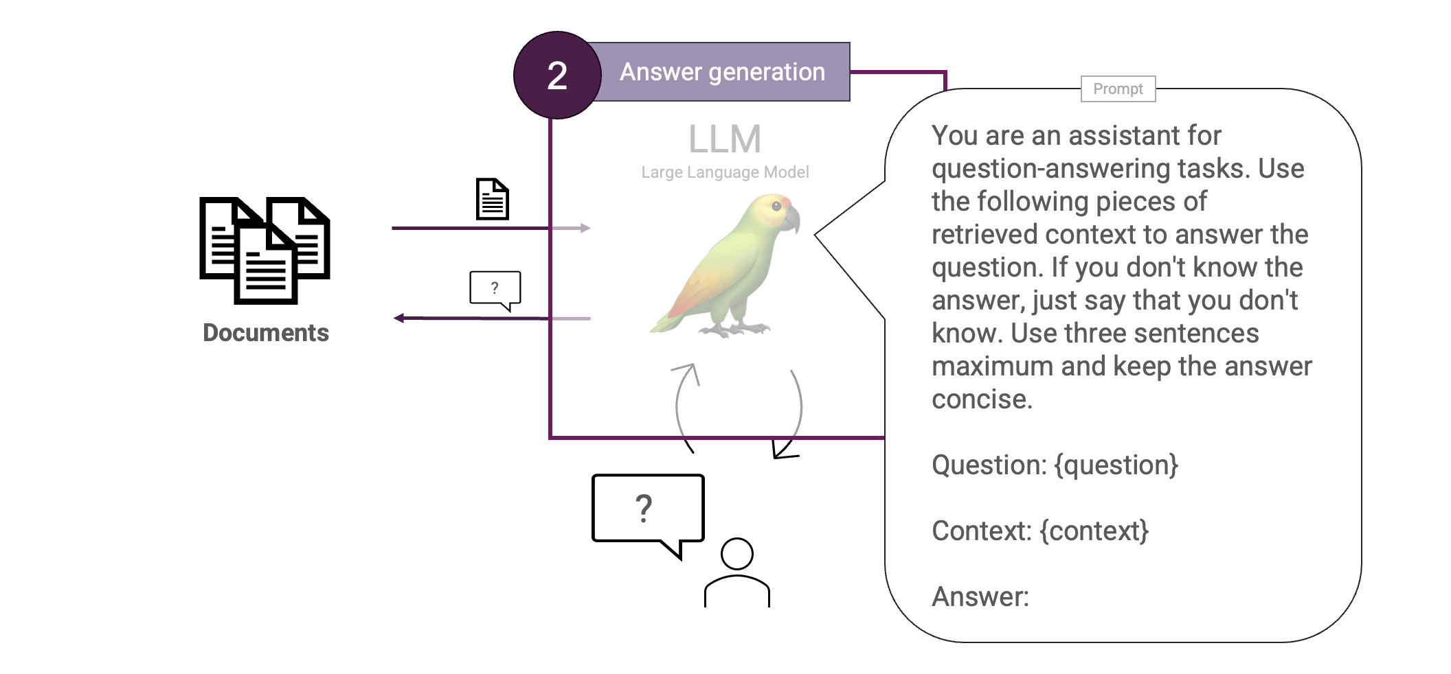
Cool. That concludes our full first version of the Basic RAG. To test our RAG system, we need some data. I recently went to PyData and figured how cool would it be to create a RAG based on their schedule. Let’s design a RAG using the schedule of PyData Eindhoven 2024.
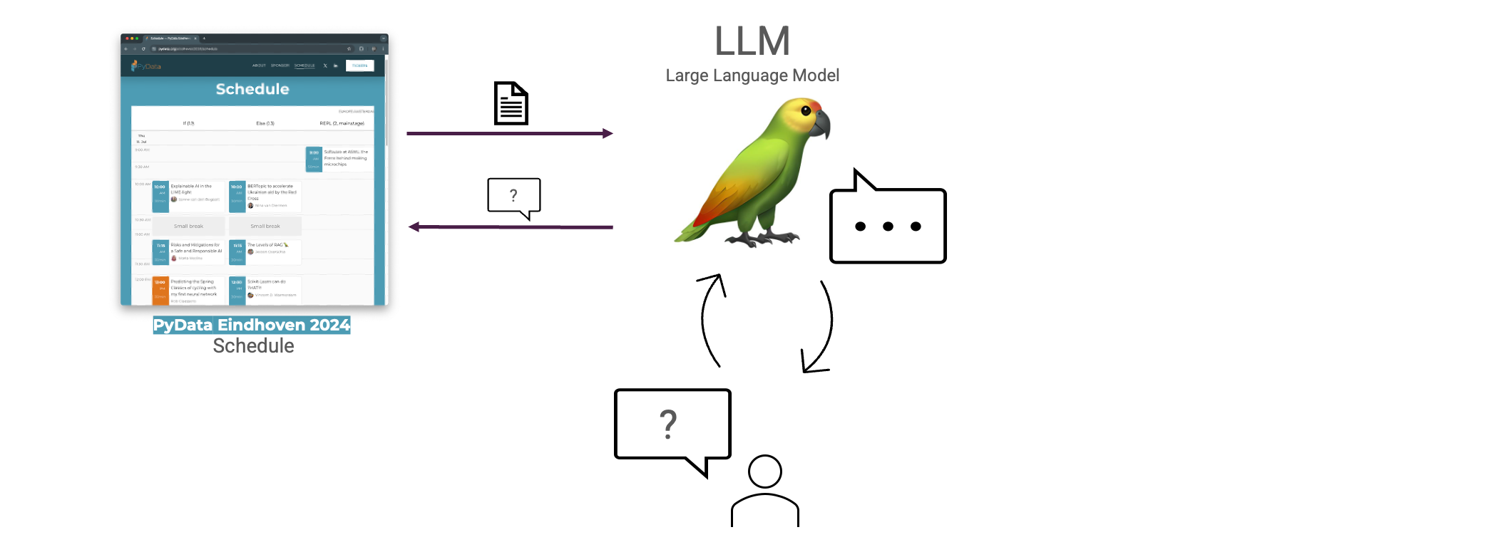
So how do we ingest such a schedule in a vector database? We will take each session and format it as Markdown, respecting the structure of the schedule by using headers.
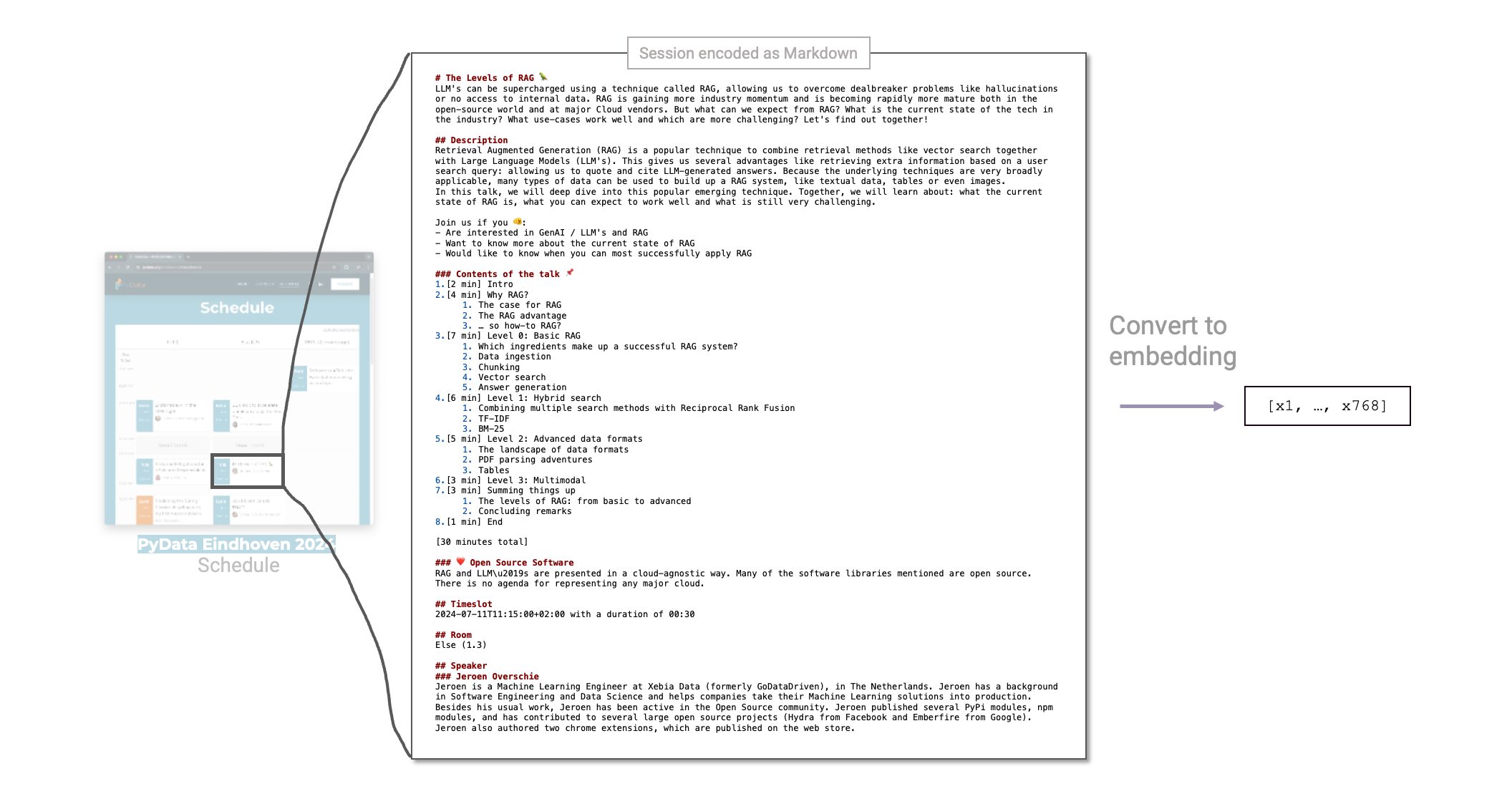
Our RAG system is now fully functional. We embedded all sessions and ingested them into a vector database. We can then find sessions similar to the user question using vector similarity search and answer the question based on a predefined prompt. Let’s test it out!
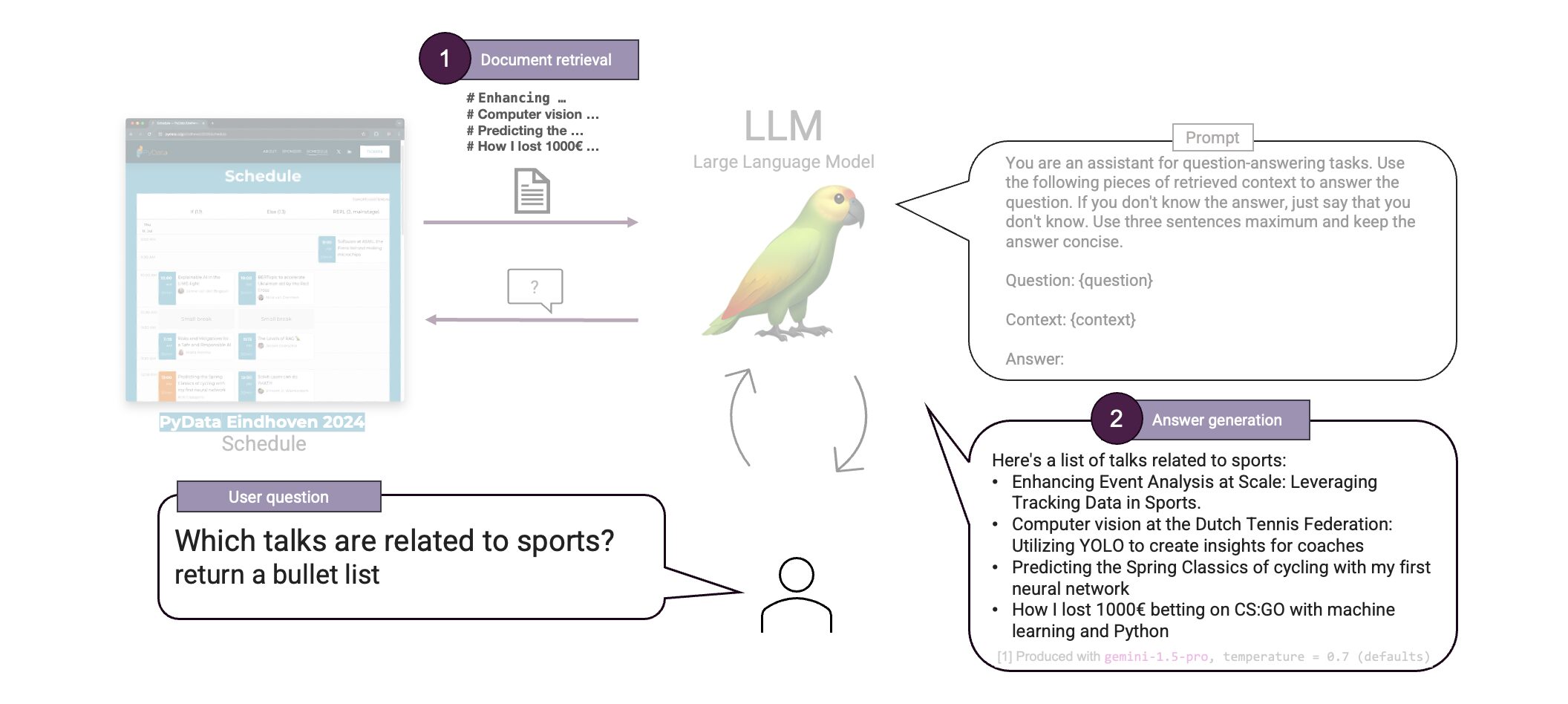
That is cool! Our RAG was able to correctly answer the question. Upon inspection of the schedule we can see that the listed talks are indeed all related to sports. We just built a first RAG system 🎉.
There are points of improvement, however. We are now embedding the sessions in its entirety. But embedding large pieces of text can be problematic, because:
- ❌ Embeddings can get saturated and lose meaning
- ❌ Imprecise citations
- ❌ Large context → high cost
So what we can do to solve this problem is to divide up text in smaller pieces, then embed those instead. This is Chunking.
Chunking
In chunking the challenge lies in determining how to divide up the text to then embed those smaller pieces. There are many ways to chunk text. Let’s first look at a simple one. We will create chunks of fixed length:

Character Text Splitter with
chunk_size = 25. This is an unrealistically small chunk size but is merely used for example sake.This is not ideal. Words, sentences and paragraphs are not respected and are split at inconvenient locations. This decreases the quality of our embeddings. We can do better than this. Let’s try another splitter that tries to better respect the structure of the text by taking into account line breaks (¶):

Recursive Character Text Splitter with
chunk_size = 25. This is an unrealistically small chunk size but is merely used for example sake.This is better. The quality of our embeddings is now better due to better splits. Note that chunk_size = 25 is only used for example sake. In practice we will use larger chunk sizes like 100, 500, or 1000. Try and see what works best on your data. But most notably, also do experiment with different text splitters. The LangChain Text Splitters section has many available and the internet is full of others.
Now we have chunked our text, we can embed those chunks and ingest them in our vector database. Then, when we let the LLM answer our question we can also ask it to state which chunks it used in answering the question. This way, we can pinpoint accurately which information the LLM was grounded in whilst answering the question, allowing us to provide the user with Citations:
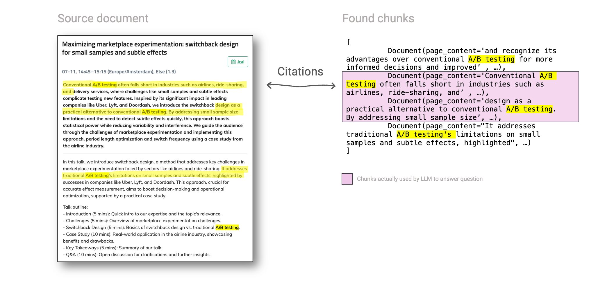
That is great. Citations can be very powerful in a RAG application to improve transparency and thereby also user trust. Summarized, chunking has the following benefits:
- Embeddings are more meaningful
- Precise citations
- Shorter context → lower cost
We can now extend our Document retrieval step with chunking:
We have our Basic RAG set up with Vector search and Chunking. We also saw our system can answer questions correctly. But how well actually does it do? Let’s take the question “What’s the talk starting with Maximizing about?” and launch it at our RAG:
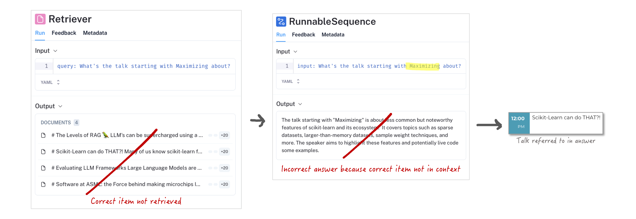
UI shown is LangSmith, a GenAI monitoring tool. Open source alternative is LangFuse.
Ouch! This answer is wildly wrong. This is not the talk starting with Maximizing. The talk described has the title Scikit-Learn can do THAT?!, which clearly does not start with the word Maximizing.
For this reason, we need another method of search, like keyword search. Because we would also still like to keep the benefits of vector search, we can combine the two methods to create a Hybrid Search.
Level 2: Hybrid Search

In Hybrid Search, we aim to combine two ranking methods to get the best of both worlds. We will combine Vector search with Keyword search to create a Hybrid Search setup. To do so, we must pick a suitable ranking method. Common ranking algorithms are:
- TF-IDF: Term Frequency-Inverse Document Frequency
- Okapi BM-25: Okapi Best Matching 25
… of which we can consider BM-25 an improved version of TF-IDF. Now, how do we combine Vector Search with an algorithm like BM-25? We now have two separate rankings we want to fuse together into one. For this, we can use Reciprocal Rank Fusion:

Reciprocal Rank Fusion is massively useful to combine two rankings. This way, we can now use both Vector search and Keyword search to retrieve documents. We can now extend again our Document retrieval step to create a Hybrid Search setup:
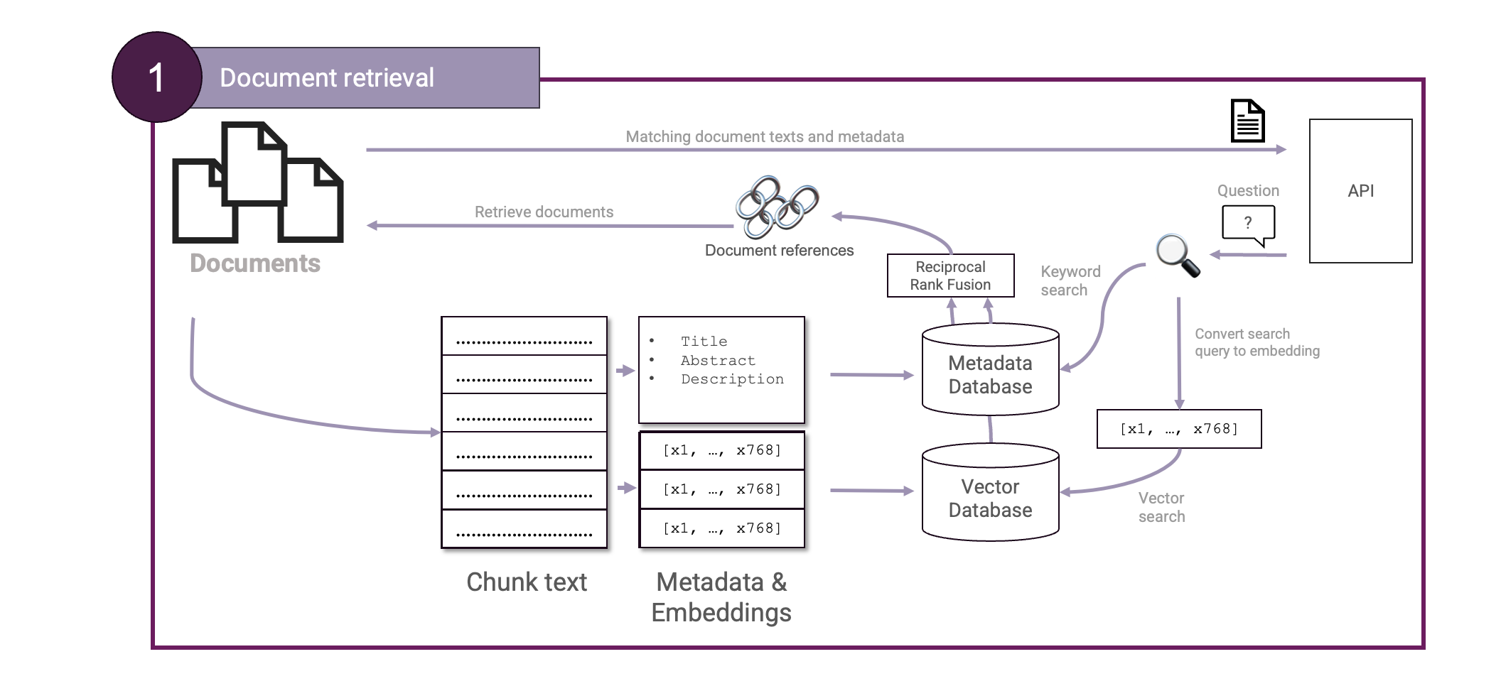
Most notably, when a user performs a search, a query is made both to our vector database and to our keyword search. Once the results are merged using Reciprocal Rank Fusion, the top results are taken and passed back to our LLM.
Let’s take again the question “What’s the talk starting with Maximizing about?” like we did in Level 1 and see how our RAG handles it with Hybrid Search:
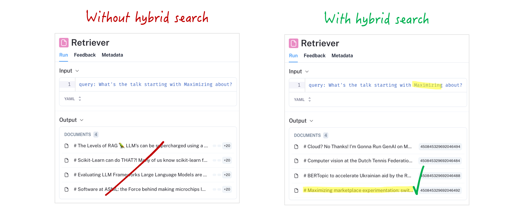
That is much better! 👏🏻 The document we were looking for was now ranked high enough that it shows up in our retrieval step. It did so by boosting the terms used in the search query. Without the document available in our prompt context, the LLM could impossibly give us the correct answer. Let’s see both the retrieval step and generation step to see what our LLM now answers on this question:
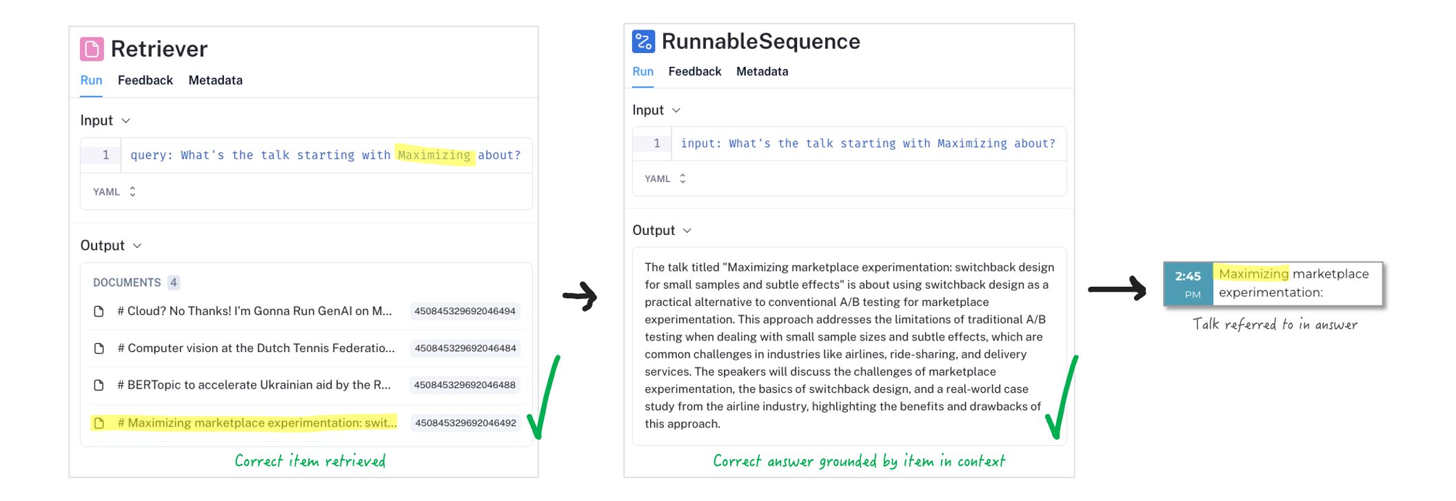
That is the correct answer ✓. With the right context available to the LLM we also get the right answer. Retrieving the right context is the most important feature of our RAG: without it, the LLM can impossibly give us the right answer.
We now learned how to build a Basic RAG system and how to improve it with Hybrid Search. The data we loaded in comes from the PyData Eindhoven 2024 schedule: which was actually conveniently available in JSON format. But what about other data formats? In the real world, we can be asked to ingest other formats into our RAG like HTML, Word, and PDF.

Formats like HTML, Word and especially PDF can be very unpredictable in terms of structure, making it hard for us to parse them consistently. PDF documents can contain images, graphs, tables, text, basically anything. So let us take on this challenge and level up to Level 3: Advanced data formats.
Level 3: Advanced data formats

This level revolves around ingesting challenging data formats like HTML, Word or PDF into our RAG. This requires extra considerations to do properly. For now, we will focus on PDF’s.
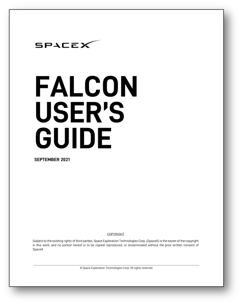
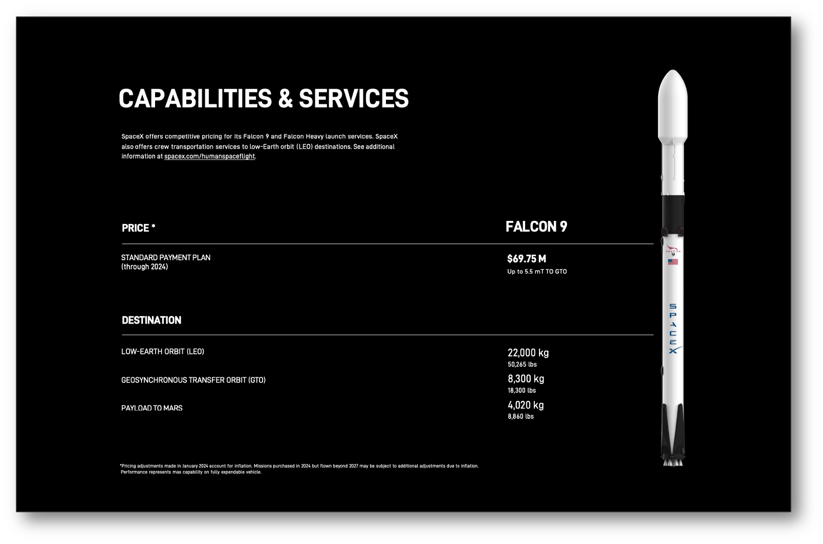
So, let us take some PDF’s as an example. I found some documents related to Space X’s Falcon 9 rocket:
 |  |  |
|---|---|---|
| User’s guide (pdf) | Cost estimates (pdf) | Capabilities & Services (pdf) |
We will now want to first parse those documents into raw text, such that we can then chunk- and embed that text. To do so, we will use a PDF parser for Python like pypdf. Conveniently, there’s a LangChain loader available for pypdf:
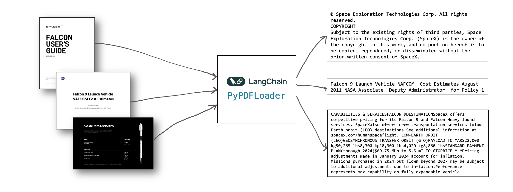
Using pypdf we could convert these PDF’s into raw text. Note there’s many more available, check out the LangChain API reference. Both offline, local and Cloud solutions are offered like GCP Document AI, Azure Document Intelligence or Amazon Textract.
With such a document parsing step set up, we will need to extend our Document retrieval step to cover this new component:

Time to test out our RAG! We embedded and ingested the raw text into our vector database and can now make queries against it. Let’s ask about the cost of a Falcon 9 rocket launch:

Awesome, that is the correct answer. Let’s try another question: “What is the payload I can carry with the Falcon 9 rocket to Mars?“:

Ow! Our RAG got that answer all wrong. It suggests we can bring double the payload to Mars than what is allowed. That is pretty inconvenient, in case you were preparing for a trip to Mars 😉.
We need to debug what went wrong. Let’s look at the context that was passed to the LLM:
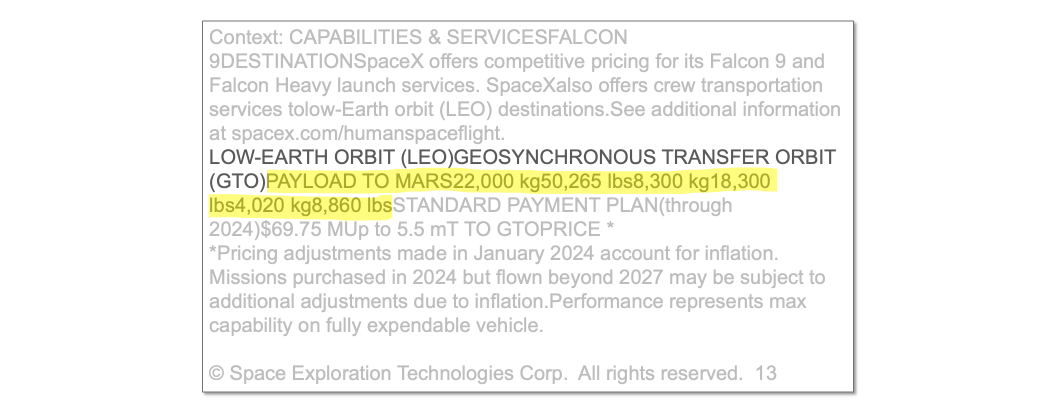
That explains a bunch. The context we’re passing to the LLM is hard to read and has a table encoded in a jumbled way. Like us the LLM has a hard time making sense of this. Therefore, we need to better encode this information in the prompt so our LLM can understand it.
If we want to support tables we can introduce an extra processing step. One option is to use Computer vision models to detect tables inside our documents, like table-transformer. If a table gets detected we can then give it a special treatment. What we can for example do, is encode tables in our prompt as Markdown:

Having detected the table and parsed it into a native format in our Python code allows us to then encode it in Markdown. Let’s pass that to our LLM instead and see what it answers this time:
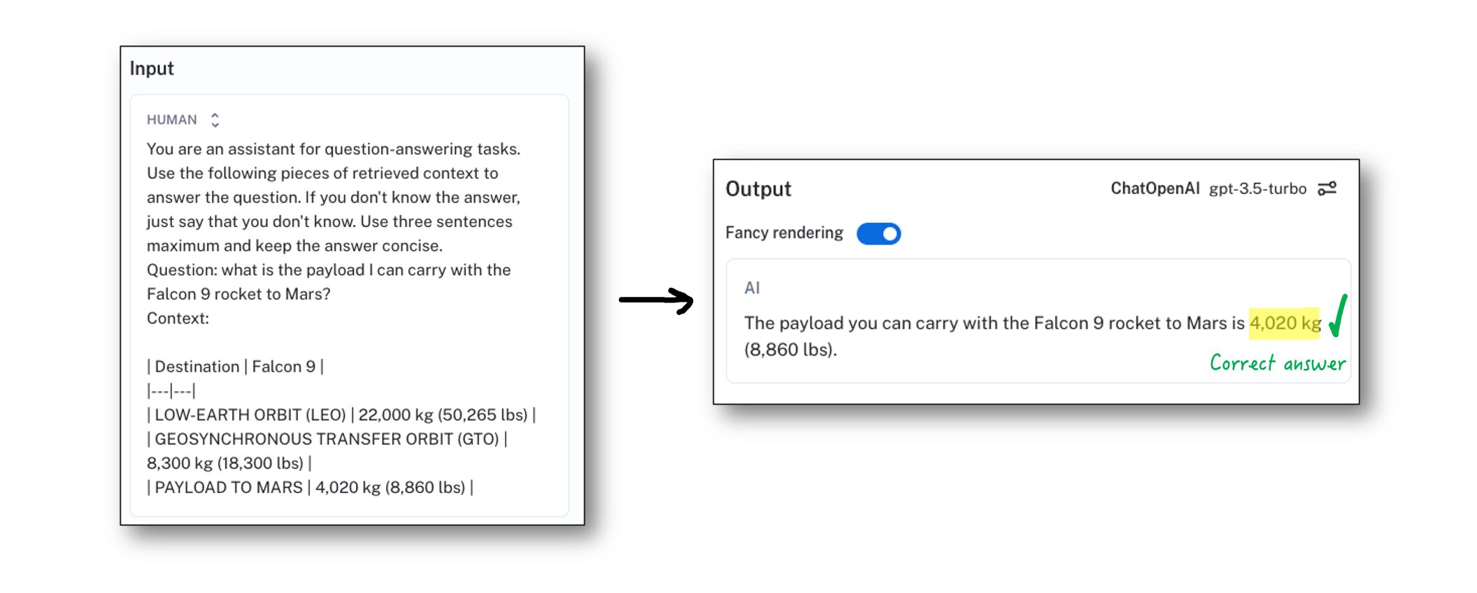
Hurray! We got it correct this time. The LLM we used could easily interpret the Markdown table and pinpoint the correct value to use in answering the question. Note that still, we need to be able to retrieve the table in our retrieval step. This setup assumes we built a retrieval step that is able to retrieve the table given the user question.
However, I have to admit something. The model we have been using for this task was GPT-3.5 turbo, which is a text-only model. Newer models have been released that can handle more than just text, which are Multimodal models. After all, we are dealing with PDF’s which can also be seen as a series of images. Can we leverage such multimodal models to better answer our questions? Let’s find out in Level 4: Multimodal.
Level 4: Multimodal

In this final level, we will look into leveraging the possibilities of Multimodal models. One of them is GPT-4o, which was announced May 2024:

This is a very powerful model that can understand audio, vision and text. This means we can feed it images as part of an input prompt. Given that we can in our retrieval step retrieve the right PDF pages to use, we can insert those images in the prompt and ask the LLM our original question. This has the advantage that we can understand content that was previously very challenging to encode in just text. Also, content we interpret and encode as text is exposed to more conversion steps exposing us to risk of information getting lost in translation.
For example sake we will take the same table we had before but then answer the question using a Multimodal model. We can take the retrieved PDF pages encoded as images and insert them right into the prompt:
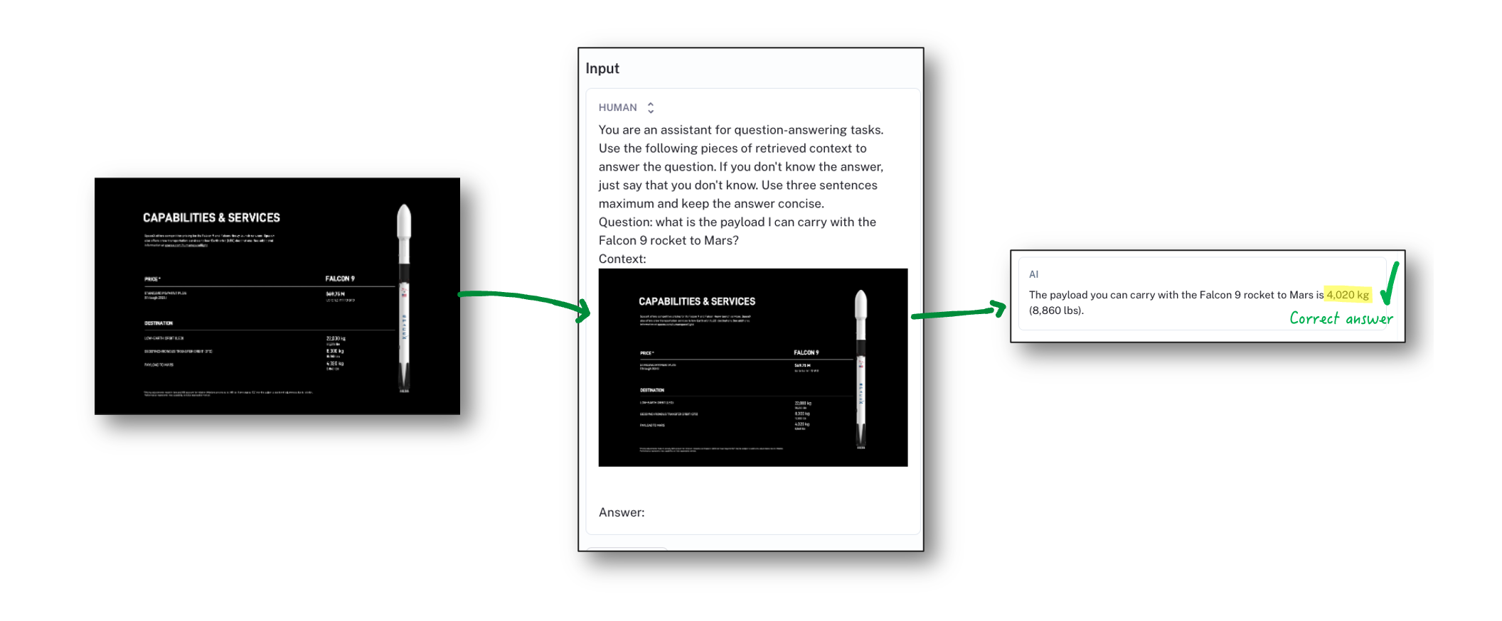
Impressive. The LLM got the answer correct. We should be aware though, that inserting images in the prompt comes with a very different token usage than the Markdown table we inserted as text before:

That is an immense increase in cost. Multimodal models can be incredibly powerful to interpret content that is otherwise very difficult to encode in text, as long as it is worth the cost ✓.
Concluding
We have explored RAG in 4 levels of complexity. We went from building our first basic RAG to a RAG that leverages Multimodal models to answer questions based on complex documents. Each level introduces new complexities which are justified in each their own way. Summarising, the Levels of RAG are:
 Level 1 Level 1Basic RAG |  Level 2 Level 2Hybrid Search |  Level 3 Level 3Advanced data formats |  Level 4 Level 4Multimodal |
|---|---|---|---|
| RAG’s main steps are 1) retrieval and 2) generation. Important components to do so are Embedding, Vector Search using a Vector database, Chunking and a Large Language Model (LLM). | Combining vector search and keyword search can improve retrieval performance. Sparse text search can be done using: TF-IDF and BM- 25. Reciprocal Rank Fusion can be used to merge two search engine rankings. | Support formats like HTML, Word and PDF. PDF can contain images, graphs but also tables. Tables need a separate treatment, for example with Computer Vision, to then expose the table to the LLM as Markdown. | Multimodal models can reason across audio, images and even video. Such models can help process complex data formats, for example by exposing PDF’s as images to the model. Given that the extra cost is worth the benefit, such models can be incredibly powerful. |
RAG is a very powerful technique which can open up many new possibilities at companies. The Levels of RAG help you reason about the complexity of your RAG and allow you to understand what is difficult to do with RAG and what is easier. So: what is your level? 🫵
We wish you all the best with building your own RAG 👏🏻.
All code available in a GitHub repository


